Lecture 6 - Primal optimization

ECE364 - Programming Methods for Machine Learning

Nickvash Kani

Slides based off prior lectures by Alex Schwing, Aigou Han, Farzas Kamalabadi, Corey Snyder. All mistakes are my own!

In this lecture we will cover:

• Basics of optimization
• Convexity
• Steepest descent
• Gradient momentum

What's primal optimization?

1. Primal Optimization Problem

• The primal problem is the original optimization problem we want to solve.
• Typically, it is formulated as a minimization or maximization problem with constraints.
• It involves decision variables, an objective function, and constraints.

Example of a Primal Problem (Convex Optimization Form) $$ \min_{x} \quad f(x) $$ $$ \text{subject to } g_i(x) \leq 0, \quad i = 1, ..., m $$ $$ h_j(x) = 0, \quad j = 1, ..., p $$ where:

• ( f(x) ) is the objective function.
• ( g_i(x) ) are inequality constraints.
• ( h_j(x) ) are equality constraints.
• ( x ) are the primal decision variables.

2. Dual Optimization Problem

• The dual problem is derived from the primal problem using Lagrange multipliers.
• Instead of optimizing over the original decision variables $x$, it optimizes over the Lagrange multipliers.
• The dual problem provides a lower bound (in minimization problems) or an upper bound (in maximization problems) to the primal solution.
• Strong duality holds under certain conditions (e.g., Slater’s condition in convex problems), meaning the primal and dual solutions are equal.

Forming the Dual Problem

We construct the Lagrangian function: $$ L(x, \lambda, \nu) = f(x) + \sum_{i=1}^{m} \lambda_i g_i(x) + \sum_{j=1}^{p} \nu_j h_j(x) $$ where:

• $\lambda_i \geq 0$ are dual variables (Lagrange multipliers) for inequality constraints.
• $\nu_j$ are dual variables for equality constraints.

The dual function is: $$ \theta(\lambda, \nu) = \inf_x L(x, \lambda, \nu) $$ Then, the dual optimization problem is: $$ \max_{\lambda \geq 0, \nu} \theta(\lambda, \nu) $$

We don't need to know about dual optimization in this course

Returning back to our optimization problem

The problem more generally: $$ \min_{x} \quad f(x) $$ $$ \text{subject to } g_i(x) \leq 0, \quad i = 1, ..., m $$

Solution: Solution $x^*$ has smallest value $f_0(w^*)$ amon gall the values that satisfythe constraints.

Questions:

• When can we find the optima?
• What algorithms are there to find the optima?
• How long does it take to find the optima?

Convexity

Understanding the Convexity Inequality

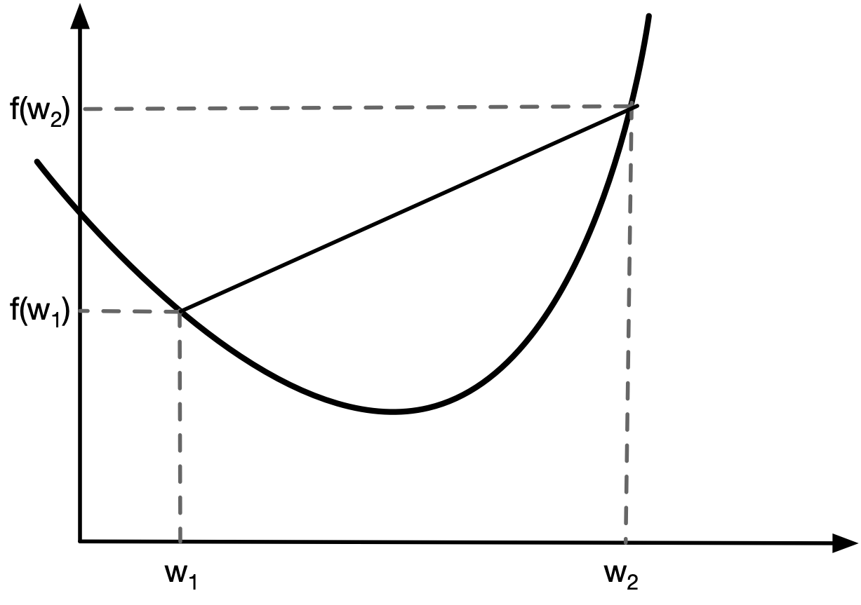
A convex function is a function where the line segment between any two points on its graph lies above or on the graph of the function. This property ensures that the function does not have "dips" or "valleys" beyond what is expected from a convex shape.

Mathematical Definition

A function $ f: \mathbb{R}^n \to \mathbb{R} $ is convex if, for all points $ x, y \in \mathbb{R}^n $ and for all $ \lambda \in [0,1] $, the following inequality holds:

$$ f(\lambda x + (1-\lambda) y) \leq \lambda f(x) + (1-\lambda) f(y) $$

This condition means that for any two points $ x $ and $ y $, the function evaluated at any convex combination of these points is less than or equal to the corresponding convex combination of function values.

Examples of Convex Functions

• Exponential: $ \exp(a x) $ is convex on $ x \in \mathbb{R} $ for all $ a \in \mathbb{R} $.
• Negative Logarithm: $ -\log(x) $ is convex on $ x \in \mathbb{R}_{++} $.
• Negative Entropy: $ -H(x) = x \log(x) $ is convex on $ x \in \mathbb{R}_{++} $.
• Norms: $ \| w \|_p $ for $ p \geq 1 $.
• Log-Sum-Exp: $ \log(\exp(w_1) + \dots + \exp(w_d)) $.

Operations Which Preserve Convexity

• Non-negative weighted sums: $ \alpha_i \geq 0 $; if $ f_i $ are convex for all $ i $, then so is:

  $$ g = \alpha_1 f_1 + \alpha_2 f_2 + \dots $$

• Composition with an affine mapping: If $ f $ is convex, then so is:

  $$ g(\mathbf{w}) = f(A\mathbf{w} + b) $$

• Pointwise maximum: If $ f_1, f_2 $ are convex, then so is:

  $$ g(\mathbf{w}) = \max \{ f_1(\mathbf{w}), f_2(\mathbf{w}) \} $$

Why is convexity important?

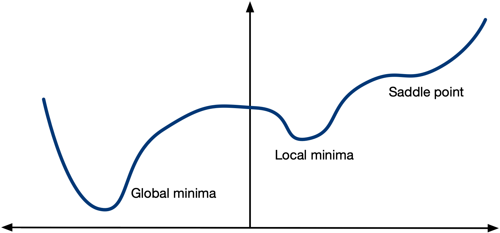
• Global Optimality Guarantee If a function is convex, any local minimum is also a global minimum. This is a crucial property because, in general, non-convex functions may have multiple local minima, making it difficult to find the best solution. Formally, for a convex function $ f(x) $, if $ x^* $ satisfies:

  $$ \nabla f(x^*) = 0 $$

  then $ x^* $ is a global minimum.

• Efficient Algorithms for Convex Problems Convex optimization problems can often be solved efficiently using well-established algorithms, including:

  • Gradient Descent (for smooth convex functions)
  • Newton’s Method (for strongly convex functions)
  • Interior-Point Methods (for constrained convex optimization)

  • Simplex and Interior-Point Methods (for convex Linear Programming problems)

    These algorithms are guaranteed to converge to the global minimum under appropriate conditions.

How do we find the minima?

Iterative Algorithm

• Start with some guess $ \mathbf{w} $
• Iterate $ k = 1, 2, 3, \dots $
  • Select direction $ d_k $ and step size $ \alpha_k $
  • Update:
    $$ \mathbf{w} \gets \mathbf{w} + \alpha_k d_k $$
  • Check whether we should stop (e.g., if $ \nabla f(\mathbf{w}) \approx 0 $)

---

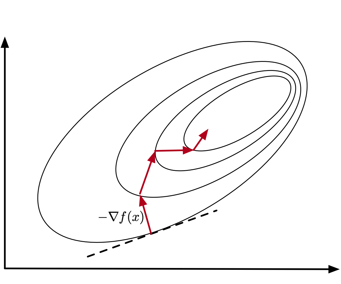
Descent Direction

The descent direction $ d_k $ satisfies:

$$ \nabla f(\mathbf{w})^\top d_k < 0 $$

How to select direction $d_k$

• Steepest Descent: $d_k = -\nabla f(w_k)$

Other directions also used:

• Scaled gradient $d_k = -D_k \nabla f(w_k)$ where $D_k$ is a scaling matrix (also called preconditioner)
• etc.

How to Select Stepsize

• Exact:
  $$ \alpha_k = \arg \min_{\alpha \geq 0} f(\mathbf{w}_k + \alpha d_k) $$

• Constant:
  $$ \alpha_k = \mathbb{R} $$

Steepest descent + constant step size is gradient descent!

So what's the problem? Can we call the lecture over? Interactive web tool

How to Select Stepsize (continued)

Optimal line search At every iteration $k$, optimal line search computes the step size $ \varepsilon_k $ as follows:

$$ \varepsilon_k = \arg \min_{\varepsilon \geq 0} f(\mathbf{x}_k + \varepsilon d_k). \tag{3.3} $$

Clearly, the above problem presumes a chosen direction of motion $ d_k $. The method searches for the value of $ \varepsilon_k $ over the half-line $ [0, \infty) $, therefore it is called optimal line search.

By this description, it is clear that optimal line search corresponds to a sequence of optimal local decisions, yielding maximum reduction of $ f $ at every iteration $ k $, given that the current state or position is $ \mathbf{x}_k $ and the descent direction has been chosen to be $ d_k $.

Solving for $ \varepsilon $ at every iteration of the gradient or steepest descent algorithms may be difficult and costly.

This motivates the Armijo rule. [1]

Armijo’s Rule in Machine Learning

Armijo’s rule is a step size selection method used in gradient-based optimization to ensure sufficient decrease in the objective function while maintaining stability. It is widely used in line search methods for optimization, particularly in gradient descent, Newton’s method, and quasi-Newton methods.

---

Armijo’s Rule for Step Size Selection Armijo’s rule uses a backtracking approach to find a suitable step size $ \alpha $:

1. Start with an initial step size $ \alpha = s $.

2. Check if the Armijo condition holds:

   $$ f(\mathbf{w}_k + \alpha d_k) - f(\mathbf{w}_k) \leq \sigma \alpha \nabla f(\mathbf{w}_k)^T d_k $$

3. If the condition does not hold, reduce $ \alpha $ using a decay factor $ \beta $:

   $$ \alpha = \beta \alpha, \quad \text{(e.g., with } \beta = 0.5) $$

4. Repeat until a suitable $ \alpha $ is found.

Armijo’s Condition The Armijo condition ensures that the function value decreases sufficiently after taking a step in the descent direction. Given an objective function $ f(\mathbf{w}) $, the step size $ \alpha $ must satisfy:

$$ f(\mathbf{w}_k + \alpha d_k) - f(\mathbf{w}_k) \leq \sigma \alpha \nabla f(\mathbf{w}_k)^T d_k $$

where:

• $ \mathbf{w}_k $ is the current iterate.
• $ d_k $ is the descent direction (e.g., $ d_k = -\nabla f(\mathbf{w}_k) $ in gradient descent).
• $ \alpha $ is the step size.
• $ \sigma \in (0,1) $ is a parameter that controls how much decrease is required (typically, $ \sigma \approx 0.1 $).

This condition ensures that:

• Ensures sufficient decrease: The left-hand side, $ f(\mathbf{w}_k + \alpha d_k) - f(\mathbf{w}_k) $, represents the actual change in the function value after taking a step.

• Bounds the decrease: The right-hand side, $ \sigma \alpha \nabla f(\mathbf{w}_k)^T d_k $, represents a fraction of the expected decrease based on the first-order Taylor approximation:

  $$ f(\mathbf{w}_k + \alpha d_k) \approx f(\mathbf{w}_k) + \alpha \nabla f(\mathbf{w}_k)^T d_k $$

  The condition ensures that the actual decrease is at least a fraction ( \sigma ) of the predicted decrease.

Using a smart step size helps stabalize gradient descent (and make things faster too!) Interactive web tool

Momentum in gradient descent

One problem with gradient descent is that it has no memory.

• If the gradient is pointing left, it'll go left.
• Next iteration if the gradient is pointing right, it goes right.
• This issue is especially bad for cases where the gradients are uneven among dimensions:

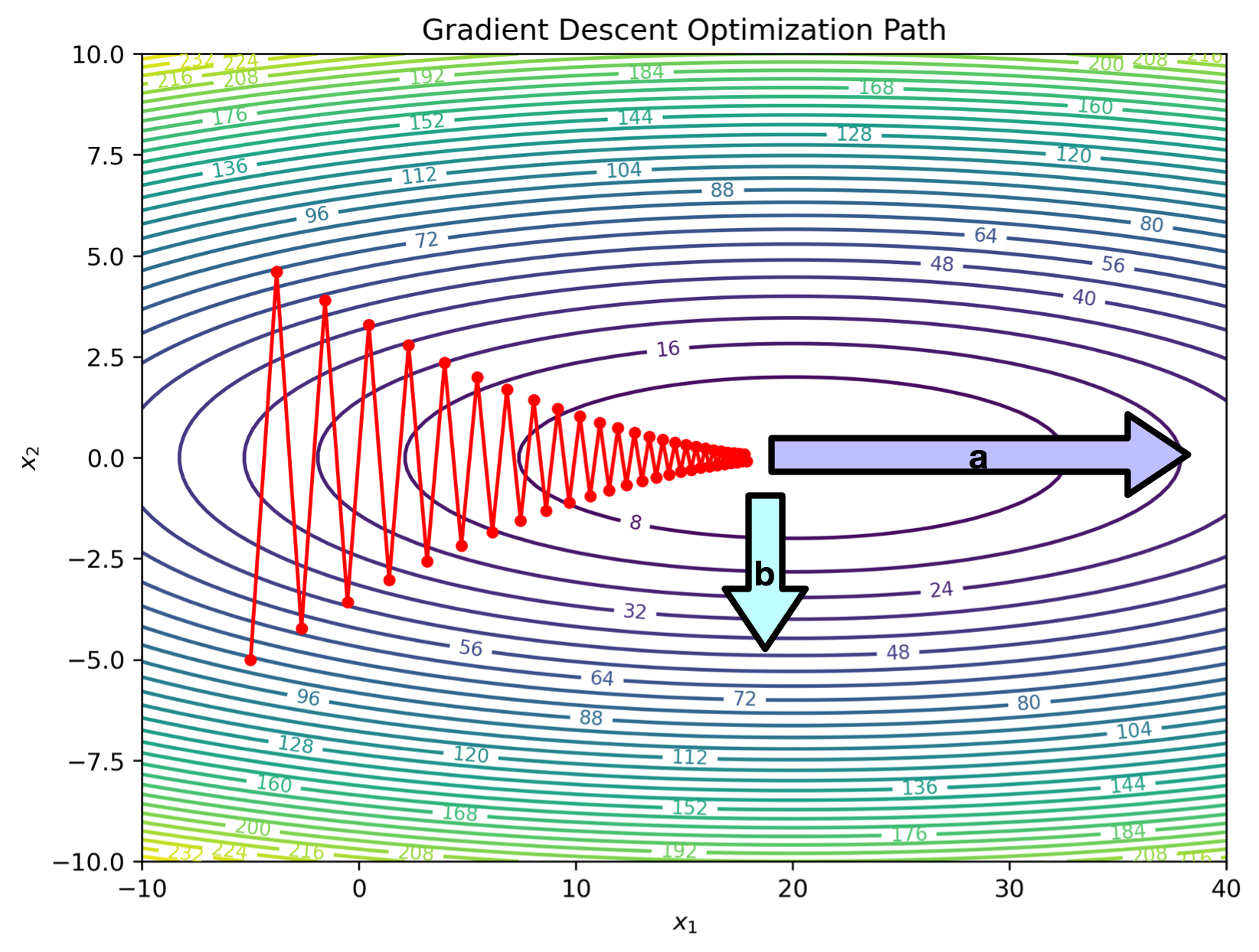
The ratio between the length of the longest and shortest principle axes of this ellipse is known as the condition number:

$$\kappa = \left(\frac{a}{b}\right)^2$$

In order to get within $\epsilon$ of a minima, we need $\geq \kappa \log\left(\frac{1}{\epsilon}\right)$ iterations Gradient Descent Condition Number Dependence

import torch
import numpy as np
import matplotlib.pyplot as plt

# Define the loss function f(x1, x2) = (x1 - 20)^2 / 20 + 2 * x2^2
def loss_function(x):
    return (x[0] - 20) ** 2 / 20 + 2 * x[1] ** 2

# Gradient of the loss function
def compute_gradient(x):
    grad_x1 = 2 * (x[0] - 20) / 20
    grad_x2 = 2 * 2 * x[1]
    return torch.tensor([grad_x1, grad_x2])

# Optimization settings
learning_rate = 0.48
iterations = 50

# Initial point
x_gd = torch.tensor([-5.0, -5.0])

# Store trajectory for plotting
gd_trajectory = [x_gd.numpy()]

# Perform optimization
for _ in range(iterations):
    grad_gd = compute_gradient(x_gd)
    x_gd = x_gd - learning_rate * grad_gd
    gd_trajectory.append(x_gd.numpy())

# Convert trajectory to NumPy for plotting
gd_trajectory = np.array(gd_trajectory)

# Create meshgrid for contour plot
x1_vals = np.linspace(-10, 40, 100)
x2_vals = np.linspace(-10, 10, 100)
X1, X2 = np.meshgrid(x1_vals, x2_vals)
Z = loss_function([X1, X2])

# Create figure and contour plot
fig, ax = plt.subplots(figsize=(8, 6))
contour = ax.contour(X1, X2, Z, levels=30, cmap='viridis')
ax.clabel(contour, inline=True, fontsize=8)

# Plot Gradient Descent trajectory
ax.plot(gd_trajectory[:, 0], gd_trajectory[:, 1], 'r-o', markersize=4, label="Gradient Descent")

# Labels and title
ax.set_xlabel('$x_1$')
ax.set_ylabel('$x_2$')
ax.set_title('Gradient Descent Optimization Path')
#ax.legend()

# Save the plot as an image file
image_filename = "./img/gradient_descent.png"
plt.savefig(image_filename, dpi=300, bbox_inches='tight')

# Show the plot
plt.show()

Gradient Descent with Momentum is an optimization algorithm that improves standard gradient descent by accelerating convergence and reducing oscillations, especially in highly curved loss landscapes.

---

Update Rule for Gradient Descent with Momentum In standard gradient descent, the update rule is:

$$ \mathbf{w}_{k+1} = \mathbf{w}_k - \alpha \nabla f(\mathbf{w}_k) $$

In gradient descent with momentum, we introduce a velocity term ( v_k ):

1. Compute the velocity (momentum update): $$ v_{k+1} = \beta v_k - \alpha \nabla f(\mathbf{w}_k) $$

2. Update weights using velocity: $$ \mathbf{w}_{k+1} = \mathbf{w}_k + v_{k+1} $$

where:

• $ \alpha $ is the learning rate.
• $ \beta \in [0,1] $ is the momentum coefficient, typically 0.9.
• $ v_k $ is the velocity term (tracks accumulated gradients).

---

Intuition Behind Momentum

• Think of momentum as a ball rolling down a hill: it builds speed in a direction and resists small changes.
• Instead of just using the current gradient, it accumulates past gradients to make updates smoother and faster.

---

Momentum Helps By:

• Accumulating past gradients to smooth updates.
• Accelerating convergence by moving in a consistent direction.
• Reducing oscillations by dampening fluctuations in gradient updates.

Gradient descent with and without momentum ($\alpha=0.2$)

Gradient descent with and without momentum ($\alpha=0.5$)

import torch
import numpy as np
import matplotlib.pyplot as plt
from mpl_toolkits.mplot3d import Axes3D

# Define the loss function f(x1, x2) = (x1 - 10)^2 / 20 + x2^2
def loss_function(x):
    return (x[0] - 20) ** 2 / 20 + 2 * x[1] ** 2

# Gradient of the loss function
def compute_gradient(x):
    grad_x1 = 2 * (x[0] - 20) / 20
    grad_x2 = 2 * 2 * x[1] ** 1
    return torch.tensor([grad_x1, grad_x2])

# Optimization settings
learning_rate = 0.2
momentum = 0.9
iterations = 50

# Initial point (starting from a far-off place)
x_gd = torch.tensor([-5.0, -5.0])
x_gdm = torch.tensor([-5.0, -5.0])

# Lists to store trajectory for plotting
gd_trajectory = [x_gd.detach().numpy()]
gdm_trajectory = [x_gdm.detach().numpy()]

# Momentum velocity term
velocity = torch.tensor([0.0, 0.0])

# Perform optimization
for _ in range(iterations):
    # Compute gradients
    grad_gd = compute_gradient(x_gd)
    grad_gdm = compute_gradient(x_gdm)

    # Normal Gradient Descent Update
    x_gd = x_gd - learning_rate * grad_gd
    gd_trajectory.append(x_gd.numpy())

    # Gradient Descent with Momentum Update
    velocity = momentum * velocity - learning_rate * grad_gdm
    x_gdm = x_gdm + velocity
    gdm_trajectory.append(x_gdm.numpy())
    
    
# Convert trajectories to NumPy for plotting
gd_trajectory = np.array(gd_trajectory)
gdm_trajectory = np.array(gdm_trajectory)

# Create a meshgrid for 3D surface plot
x1_vals = np.linspace(-10, 40, 100)
x2_vals = np.linspace(-10, 10, 100)
X1, X2 = np.meshgrid(x1_vals, x2_vals)
Z = loss_function([X1,X2])

# Plot the function surface and optimization paths
fig = plt.figure(figsize=(12, 8))

# 3D surface plot
ax = fig.add_subplot(111, projection='3d')
ax.plot_surface(X1, X2, Z, cmap='viridis', alpha=0.7)

# Plot GD trajectory
ax.plot(gd_trajectory[:, 0], gd_trajectory[:, 1], color='red', marker='o', markersize=4, label='Gradient Descent')

# Plot GDM trajectory
ax.plot(gdm_trajectory[:, 0], gdm_trajectory[:, 1], color='blue', marker='o', markersize=4, label='Momentum Gradient Descent')

# Labels and legend
ax.set_xlabel('$x_1$')
ax.set_ylabel('$x_2$')
ax.set_zlabel('Loss')
ax.set_title('Gradient Descent vs Momentum Gradient Descent')
ax.legend()

# 2D Contour plot projection
ax.contour(X1, X2, Z, levels=20, cmap='gray', zdir='z', offset=np.min(Z))

plt.show()

import torch
import numpy as np
import matplotlib.pyplot as plt
from mpl_toolkits.mplot3d import Axes3D
import matplotlib.animation as animation

# Define the loss function f(x1, x2) = (x1 - 20)^2 / 20 + 2 * x2^2
def loss_function(x):
    return (x[0] - 20) ** 2 / 20 + 2 * x[1] ** 2

# Gradient of the loss function
def compute_gradient(x):
    grad_x1 = 2 * (x[0] - 20) / 20
    grad_x2 = 2 * 2 * x[1]
    return torch.tensor([grad_x1, grad_x2])

# Optimization settings
learning_rate = 0.5
momentum = 0.9
iterations = 50

# Initial points
x_gd = torch.tensor([-5.0, -5.0])
x_gdm = torch.tensor([-5.0, -5.0])

# Lists to store trajectory for plotting
gd_trajectory = [x_gd.numpy()]
gdm_trajectory = [x_gdm.numpy()]

# Momentum velocity term
velocity = torch.tensor([0.0, 0.0])

# Perform optimization
for _ in range(iterations):
    grad_gd = compute_gradient(x_gd)
    grad_gdm = compute_gradient(x_gdm)

    # Normal Gradient Descent Update
    x_gd = x_gd - learning_rate * grad_gd
    gd_trajectory.append(x_gd.numpy())

    # Gradient Descent with Momentum Update
    velocity = momentum * velocity - learning_rate * grad_gdm
    x_gdm = x_gdm + velocity
    gdm_trajectory.append(x_gdm.numpy())

# Convert trajectories to NumPy for plotting
gd_trajectory = np.array(gd_trajectory)
gdm_trajectory = np.array(gdm_trajectory)

# Create meshgrid for surface and contour plots
x1_vals = np.linspace(-10, 40, 100)
x2_vals = np.linspace(-10, 10, 100)
X1, X2 = np.meshgrid(x1_vals, x2_vals)
Z = loss_function([X1, X2])

# Create figure and subplots
fig = plt.figure(figsize=(12, 8))

# 3D surface plot
ax3d = fig.add_subplot(121, projection='3d')
ax3d.plot_surface(X1, X2, Z, cmap='viridis', alpha=0.7)

# 2D contour plot
ax2d = fig.add_subplot(122)
contour = ax2d.contour(X1, X2, Z, levels=30, cmap='viridis')
ax2d.clabel(contour, inline=True, fontsize=8)

# Initialize points for animation
gd_point_3d, = ax3d.plot([], [], [], 'ro', markersize=8, label="Gradient Descent")
gdm_point_3d, = ax3d.plot([], [], [], 'bo', markersize=8, label="Momentum GD")

gd_point_2d, = ax2d.plot([], [], 'ro', markersize=8)
gdm_point_2d, = ax2d.plot([], [], 'bo', markersize=8)

# Plot initial trajectories
gd_traj_2d, = ax2d.plot([], [], 'r-', alpha=0.5)
gdm_traj_2d, = ax2d.plot([], [], 'b-', alpha=0.5)

# Labels and legends
ax3d.set_xlabel('$x_1$')
ax3d.set_ylabel('$x_2$')
ax3d.set_zlabel('Loss')
ax3d.set_title('Gradient Descent vs Momentum (3D Surface)')
ax3d.legend()

ax2d.set_xlabel('$x_1$')
ax2d.set_ylabel('$x_2$')
ax2d.set_title('Optimization Path on Contour')

def update(frame):
    if frame < len(gd_trajectory):
        # Update ball positions (must pass lists or arrays, not scalars)
        gd_point_3d.set_data([gd_trajectory[frame, 0]], [gd_trajectory[frame, 1]])
        gd_point_3d.set_3d_properties([loss_function(gd_trajectory[frame])])

        gdm_point_3d.set_data([gdm_trajectory[frame, 0]], [gdm_trajectory[frame, 1]])
        gdm_point_3d.set_3d_properties([loss_function(gdm_trajectory[frame])])

        gd_point_2d.set_data([gd_trajectory[frame, 0]], [gd_trajectory[frame, 1]])
        gdm_point_2d.set_data([gdm_trajectory[frame, 0]], [gdm_trajectory[frame, 1]])

        # Update trajectory lines on contour plot
        gd_traj_2d.set_data(gd_trajectory[:frame+1, 0], gd_trajectory[:frame+1, 1])
        gdm_traj_2d.set_data(gdm_trajectory[:frame+1, 0], gdm_trajectory[:frame+1, 1])

    return gd_point_3d, gdm_point_3d, gd_point_2d, gdm_point_2d, gd_traj_2d, gdm_traj_2d

# Create and save animation
ani = animation.FuncAnimation(fig, update, frames=iterations, interval=150, blit=True)

# Save the animation as a GIF file
gif_filename = "./img/gradient_vs_momentum.gif"
ani.save(gif_filename, writer=animation.PillowWriter(fps=10))

print(f"Animation saved as {gif_filename}")

Animation saved as ./img/gradient_vs_momentum.gif

That's it for today

We'll discuss linear regression next time

Other References:

[1] Dimitrios Katselis "Lecture 3: Steepest and Gradient Descent-Part I" link

[2] Lewis Mitchell, "Gradient descent: steepest descent" video

[3] Visually Explained, "Accelerate Gradient Descent with Momentum" video