In this lecture:
nn.Module object.nn.Module. nn.Module object.To recap what we have been doing for the last 2 weeks. We have:
Example:
In binary logistic regression we have:
self identifier represents the instance of the class. By using the self keyword we can access the attributes and methods of the class in python or assign attributes of the given object within the class definition. __init__ method is a reseved method in Python classes. It is known as the constructor in object oriented programming . This method called when an object is created from the class and it allow the class to initialize the attributes of a class.nn.Module class¶The nn.Module class is the universal base class for neural networks, and more broadly trainable models, in PyTorch found within the torch.nn package, i.e. torch.nn.Module. We create our own models by inheriting this base class and implementing the necessary methods for the class. There are two methods which must be implemented: __init__ and forward.
The __init__ method specifies the constructor and thus how every instance of this module must be initialized the __init__ method must first call super().__init__() to call the constructor of the base nn.Module class (and thus access all the helpful attributes and methods within). The forward method implements how the model processes input data for its forward pass.
As an example nn.Module class. Consider a class for implementing third-order polynomial regression. In this case, we have
$$
f_\theta(x) = ax^3+bx^2+cx+d
$$
and $\theta=\{a, b, c, d\}$. The corresponding nn.Module class may be written as follows.
import torch
import torch.nn as nn

class ThirdOrderPolynomial(nn.Module):
    def __init__(self):
        '''
        Specify the learnable parameters: a, b, c, d
        '''
        super().__init__() # call nn.Module constructor first
        self.a = nn.Parameter(torch.rand(1))
        self.b = nn.Parameter(torch.rand(1))
        self.c = nn.Parameter(torch.rand(1))
        self.d = nn.Parameter(torch.rand(1))

    def forward(self, x):
        '''
        Implement f(x).
        '''
        f_x = self.a*x**3 + self.b*x**2 + self.c*x + self.d
        return f_x

# create ThirdOrderPolynomial object
my_model = ThirdOrderPolynomial()
# print model parameters
print(my_model.a)
print(my_model.b)
print(my_model.c)
print(my_model.d)
x_input = torch.tensor([1])
prediction = my_model(x_input)
print(prediction)
Parameter containing:
tensor([0.4425], requires_grad=True)
Parameter containing:
tensor([0.7631], requires_grad=True)
Parameter containing:
tensor([0.3068], requires_grad=True)
Parameter containing:
tensor([0.8226], requires_grad=True)
tensor([2.3350], grad_fn=<AddBackward0>)
Important things to note:
self parameter must be used to access class attributes and methods. self not needed? nn.Parameter class.nn.Module class automatically collects all learnable paramters in the .parameters() attribute. This makes scaling our models and learning algorithms dramatically easier!In lecture notes:
self is not needed for static methods (normal functions defined inside a class for organizational purposes.¶learnable_parameters = my_model.parameters()
print(learnable_parameters)
for p in learnable_parameters:
print(p)
<generator object Module.parameters at 0x10ab518c0>
Parameter containing:
tensor([0.4425], requires_grad=True)
Parameter containing:
tensor([0.7631], requires_grad=True)
Parameter containing:
tensor([0.3068], requires_grad=True)
Parameter containing:
tensor([0.8226], requires_grad=True)
Implement a logistic regression model class for inputs $x_i\in\mathbb{R}^N$ and include a bias term. Recall that $$ f_\theta(x)=\mathbf{Pr}\{y=1|x\}=\frac{1}{1+e^{-(w^\top x+b)}}. $$
import torch
import torch.nn as nn
import numpy as np
import matplotlib.pyplot as plt

class LogisticRegression(nn.Module):
    def __init__(self, N):
        super().__init__()
        self.w = nn.Parameter(torch.ones(N))
        self.b = nn.Parameter(torch.zeros(1))

    def forward(self, x):
        return 1/(1+torch.exp(-(self.w@x+self.b)))

N = 1
my_logreg = LogisticRegression(N)
x = torch.randn(N)
y = my_logreg(x)

# Plot both on the same figure
L = 100
x_values = torch.linspace(-5, 5, L)
with torch.no_grad():
    y_values = [my_logreg(torch.tensor(x_values[i].view(1, -1))) for i in range(L)]

plt.figure(figsize=(7,5))
plt.plot(x_values.detach().numpy(), y_values, 'b', label="Logistic Function")

# Axis labels, legend, grid, etc.
plt.xlabel('x')
plt.ylabel('$\sigma$')
plt.grid(True, alpha=0.3)
plt.legend()
plt.ylim([0, 1.2])  # Adjust as needed
plt.show()
#plt.savefig("img/log_ce_loss_plot.png")
/var/folders/r5/0w7y2nzn6z519vv67rcw3ffr0000gn/T/ipykernel_74221/1862126608.py:24: UserWarning: To copy construct from a tensor, it is recommended to use sourceTensor.clone().detach() or sourceTensor.clone().detach().requires_grad_(True), rather than torch.tensor(sourceTensor).
  y_values = [my_logreg(torch.tensor(x_values[i].view(1, -1))) for i in range(L)]

Also within the torch.nn package is a variety of loss functions implemented as classes. Thus, we may create instances of these loss functions with varying attributes that may be called while training models. Most of the functions are simply wrapper functions for functions within torch.nn.functional; however, they provide a helpful interface to simplify training code.
For example, the nn.MSELoss class implements mean squared error loss with an attribute to specify the "reduction" of the loss. This reduction parameter allows us to specify if we want the squared errors to be summed, averaged, or left as a tensor of squared errors. In the latter case, we may use this to only incorporate select squared errors, i.e. masking or re-weighting, for certain applications.
In general, for model object named model, inputs named inputs, ground-truths named targets, and loss function object named criterion, we may succinctly compute the current loss for our model as follows.
predictions = model(inputs)
loss = criterion(predictions, targets)
The result of such a loss function can then act as the seed node from which we backpropagate for model training. Similarly, we may implement a custom loss function ourself (as an nn.Module class or as a regular function).
import torch
import torch.nn as nn

criterion_mean = nn.MSELoss(reduction='mean')
criterion_sum = nn.MSELoss(reduction='sum')
criterion_none = nn.MSELoss(reduction='none')

pred = torch.zeros(4)
targets = torch.ones(4)

print(criterion_mean(pred, targets))
print(criterion_sum(pred, targets))
print(criterion_none(pred, targets))
tensor(1.)
tensor(4.)
tensor([1., 1., 1., 1.])
torch.optim package¶We now know how to create a PyTorch model and how to apply a loss function to a dataset and model outputs. We have previously seen how to use the .backward() method to initiate backpropagation. However, we found it quite tedious to update each individual parameter by gradient descent and to clear those gradients each iteration.
The torch.optim package contains many helpful optimizers, i.e. learning algorithms, and other useful interfaces to simplify the parameter updating process. The simplest optimizer in the torch.optim package is the optim.SGD, which implements stochastic gradient descent (SGD). Also known as mini-batch gradient descent, SGD implements gradient descent except only computes the gradient over a random subset, or mini-batch, of the data. Thus, the computed gradient depends on a stochastic sample of the dataset. If the batch size for SGD is the entire dataset, then SGD simply becomes ordinary gradient descent.
Pros:
Cons:
The optim.SGD optimizer implements other helpful features aside from basic gradient descent including momentum and weight decay. As mentioned above, the gradients from SGD may be noisy and susceptible to random outliers. Momentum is one way to smooth out gradient descent updates by incorporating a moving average of previous gradients. Let $\mu\in[0, 1)$ be the momentum parameter, $g^{(k)}$ be the gradient over the batch in iteration $k$, and $\theta^{(k)}$ be the model parameters as iteration $k$. The learning algorithm for SGD with momentum and learning rate $\alpha$ is then
Thus, the gradients become as exponential moving average of previous gradients where all previous gradients contribute a weight of $\mu^{k-m}$ from step $m$. Popular choices of $\mu$ are larger values such as $0.9$ and $0.99$ so that the exponential moving average does not vanish too quickly.
The weight decay parameter implements the same $L_2$ regularization we saw with linear regression. For loss function $\ell(f_\theta(x), y)$ and weight decay parameter $\lambda$, the effective total loss function used for backpropagation is given by
$$ \ell_{\textrm{total}} = \ell(f_\theta(x), y)+\frac{\lambda}{2}\lVert\theta\rVert_2^2. $$Thus, an additional component of $\lambda\theta$ is added to the gradient. The purpose of weight decay is to encourage model parameters to not be too large and thus prone to overfitting and dangerous outlier behavior. Common choices of weight decay vary by model type and size, however, a small value like $10^{-5}$ is often a safe starting point. Other parameters exist within the optim.SGD class, but these two are the most important to explain.
The torch.optim package contains many other popular optimizers, such as Adagrad and Adam, which are popular adaptive gradient methods where per-layer learning rates are automatically tuned during training. For now, we will focus on applying SGD.
To initialize the SGD optimizer, and most other optimizers, we need to give the optimizer:
model.parameters() from our nn.Module object instance.import torch
optimizer = torch.optim.SGD(my_logreg.parameters(), lr=1e-3, momentum=0.99, weight_decay=1e-4)
Lastly, the overall learning rate for a learning algorithm is commonly adjusted in practice.
The most common method for this is to simply lower the learning rate by some factor whenever the loss function or validation performance appears to plateau.
The intuition for this is that a smaller learning rate allows us to more carefully descend into the current local minimum the model is converging to and hopefully provide additional modest improvements in performance.
The torch.optim package provides helpful learning rate scheduler interfaces where different learning rate policies may be implemented, e.g. after some number of gradient descent updates, after loss plateaus, or different policies for variably increasing or decreasing the learning rate. We will not worry about these for now, but they are important to point out within this package.
Finally, we have all the necessary ingredients to create a PyTorch training loop! This training loop, while basic, forms the core of any model training code within PyTorch. Before executing the training loop, we need to ensure a few things are set:
With these in hand, the training loop takes on the following basic cycle for optimizer named optimizer and loss function named criterion:
optimizer.zero_grad().criterion.optimizer.step()And that's it! Let's get some practice with a toy dataset.
import torch
import torch.nn as nn
import numpy as np
import matplotlib.pyplot as plt
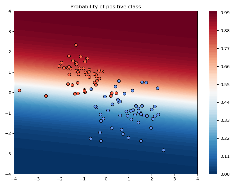
# plotting utility function to visualize model proabilities of positive class
def plot_model_probs(model, plus_class, negative_class):
x = torch.linspace(-4, 4, 100)
y = torch.linspace(-4, 4, 100)
X, Y = torch.meshgrid(x, y, indexing='ij')
meshgrid_inputs = torch.stack((X.flatten(), Y.flatten()), dim=1).unsqueeze(-1)
with torch.no_grad():
meshgrid_outputs = logreg_model(meshgrid_inputs)
plt.figure(figsize=(8, 6))
plt.contourf(X.numpy(), Y.numpy(), meshgrid_outputs.reshape(100, 100).numpy(), cmap='RdBu_r', levels=100)
plt.colorbar()
plt.title('Probability of positive class')
plt.scatter(plus_class[:, 0].numpy(), plus_class[:, 1].numpy(), color='tomato', s=50, edgecolor='black')
plt.scatter(negative_class[:, 0].numpy(), negative_class[:, 1].numpy(), color='cornflowerblue', s=50, edgecolor='black')
plt.tight_layout()
# compute classification accuracy
def model_accuracy(model, input_data, labels):
predictions = model(input_data.unsqueeze(-1)).squeeze(-1)
positive_preds = predictions >= 0.5
negative_preds = predictions < 0.5
n_correct = torch.sum(positive_preds*labels)+torch.sum(negative_preds*(1-labels))
return n_correct/len(labels)
# prepare dataset
N = 50 # 50 points per class
plus_class = 0.75*torch.randn(N, 2) + torch.tensor([-1, 1])
negative_class = 0.75*torch.randn(N, 2) + torch.tensor([1, -1])
input_data = torch.cat((plus_class, negative_class), dim=0)
labels = torch.cat((torch.ones(N), torch.zeros(N)))
print(input_data.shape, labels.shape)
plt.figure(figsize=(8, 6))
plt.scatter(plus_class[:, 0].numpy(), plus_class[:, 1].numpy(), color='tomato', s=50, edgecolor='black')
plt.scatter(negative_class[:, 0].numpy(), negative_class[:, 1].numpy(), color='cornflowerblue', s=50, edgecolor='black')
plt.tight_layout()
torch.Size([100, 2]) torch.Size([100])

# setup before training loop
# set up model
logreg_model = LogisticRegression(2)

# loss function and optimizer
criterion = nn.BCELoss(reduction='mean') # binary cross-entropy loss, use mean loss
lr = 1e-2 # learning rate
optimizer = torch.optim.SGD(logreg_model.parameters(), lr=lr)

# plotting utility, initial model performance (before learning!)
plot_model_probs(logreg_model, plus_class, negative_class) # initial
print('Model accuracy: {:.3f}'.format(model_accuracy(logreg_model, input_data, labels)))
Model accuracy: 0.510

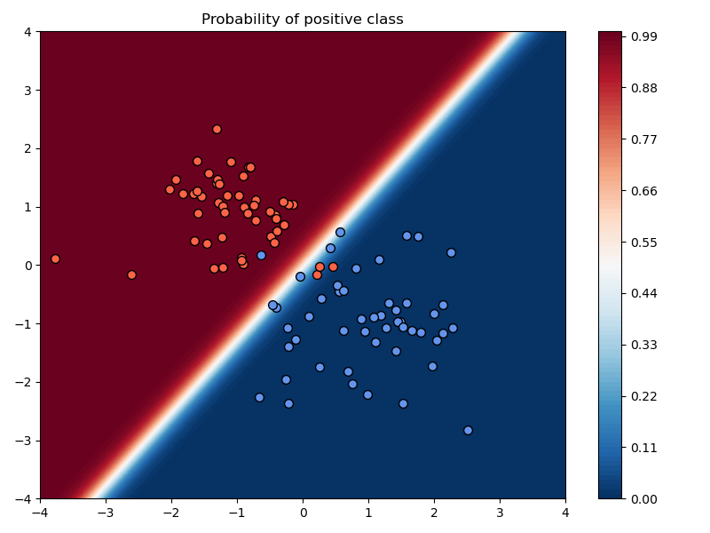
In the above example, we chose a learning rate of $\alpha=10^{-2}$, used no momentum, used no weight decay, and trained the model for 200 iterations.
Compare the results of training with and without momentum, keeping the learning rate and number of iterations fixed.
# Part a)
# loss function and optimizer
criterion = nn.BCELoss(reduction='mean') # binary cross-entropy loss, use mean loss
lr = 1e-2 # learning rate
# without momentum
plot_probs = True
logreg_model = LogisticRegression(2)
optimizer = torch.optim.SGD(logreg_model.parameters(), lr=lr)
# training loop
n_iter = 200
batch_size = 16
loss_values, accuracies = [], []
for n in range(n_iter):
# zero out gradients
optimizer.zero_grad()
# sample random batch and pass to model
batch_indices = np.random.choice(np.arange(len(labels)), size=batch_size)
input_batch = input_data[batch_indices].unsqueeze(-1) # make dimensions match for matrix multiplication
label_batch = labels[batch_indices]
predictions = logreg_model(input_batch).squeeze(-1) # make dimensions match for loss function
# calculate loss
loss = criterion(predictions, label_batch)
# backpropagate and update
loss.backward()
optimizer.step()
# logging
loss_values.append(loss.item())
accuracies.append(model_accuracy(logreg_model, input_data, labels))
# plot model probabilities
if plot_probs:
plot_model_probs(logreg_model, plus_class, negative_class)
plt.savefig("./img/classification_no_momentum.png")
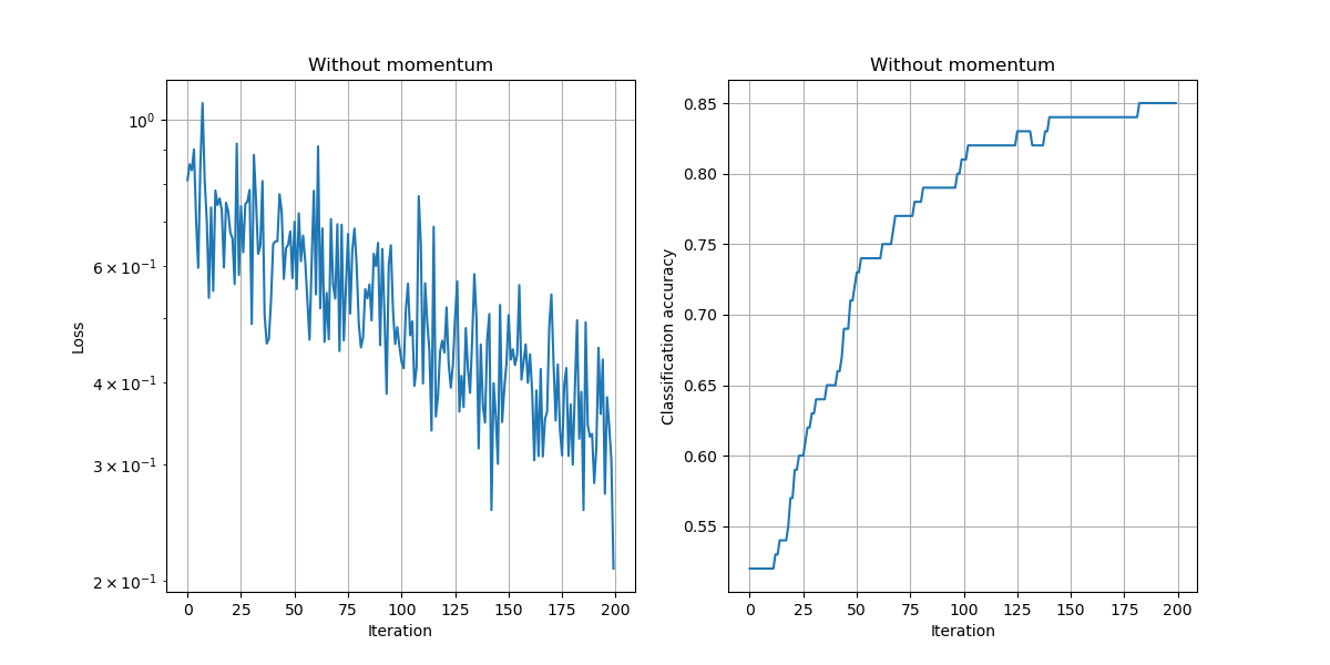
# plot loss values
plt.figure(figsize=(12,6))
plt.subplot(121)
plt.semilogy(loss_values)
plt.grid(True)
plt.title('Without momentum')
plt.xlabel('Iteration')
plt.ylabel('Loss')
plt.subplot(122)
plt.plot(accuracies)
plt.grid(True)
plt.title('Without momentum')
plt.xlabel('Iteration')
plt.ylabel('Classification accuracy')
plt.savefig("./img/lossacc_no_momentum.png")
# with momentum
plot_probs = True
logreg_model = LogisticRegression(2) # re-initialize model
optimizer = torch.optim.SGD(logreg_model.parameters(), lr=lr, momentum=0.99)
# training loop
n_iter = 200
batch_size = 16
loss_values, accuracies = [], []
for n in range(n_iter):
# zero out gradients
optimizer.zero_grad()
# sample random batch and pass to model
batch_indices = np.random.choice(np.arange(len(labels)), size=batch_size)
input_batch = input_data[batch_indices].unsqueeze(-1) # make dimensions match for matrix multiplication
label_batch = labels[batch_indices]
predictions = logreg_model(input_batch).squeeze(-1) # make dimensions match for loss function
# calculate loss
loss = criterion(predictions, label_batch)
# backpropagate and update
loss.backward()
optimizer.step()
# logging
loss_values.append(loss.item())
accuracies.append(model_accuracy(logreg_model, input_data, labels))
# plot model probabilities
if plot_probs:
plot_model_probs(logreg_model, plus_class, negative_class)
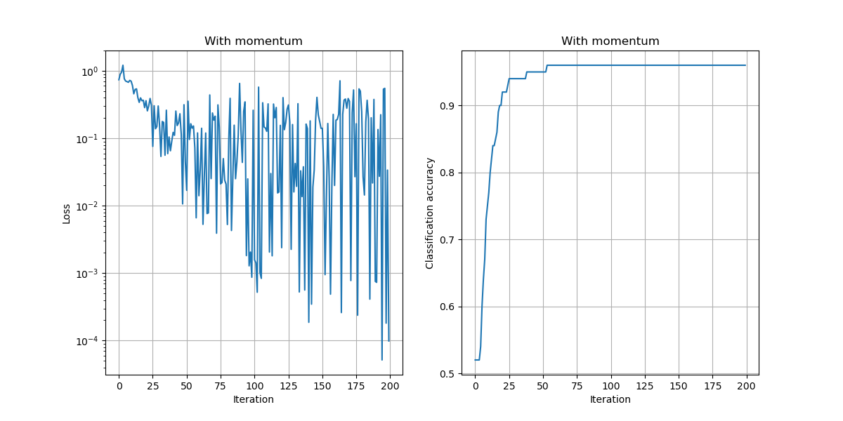
plt.savefig("./img/classification_w_momentum.png")
# plot loss values
plt.figure(figsize=(12,6))
plt.subplot(121)
plt.semilogy(loss_values)
plt.grid(True)
plt.title('With momentum')
plt.xlabel('Iteration')
plt.ylabel('Loss')
plt.subplot(122)
plt.plot(accuracies)
plt.grid(True)
plt.title('With momentum')
plt.xlabel('Iteration')
plt.ylabel('Classification accuracy')
plt.savefig("./img/lossacc_w_momentum.png")


 |
 |
 |
 |
Setting:
Observations:
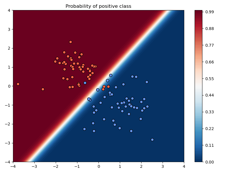
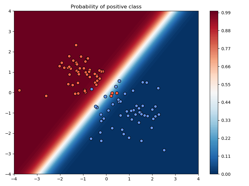
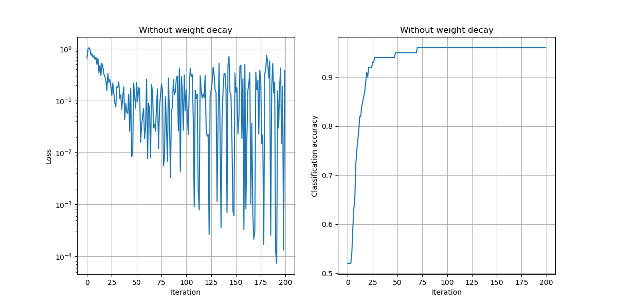
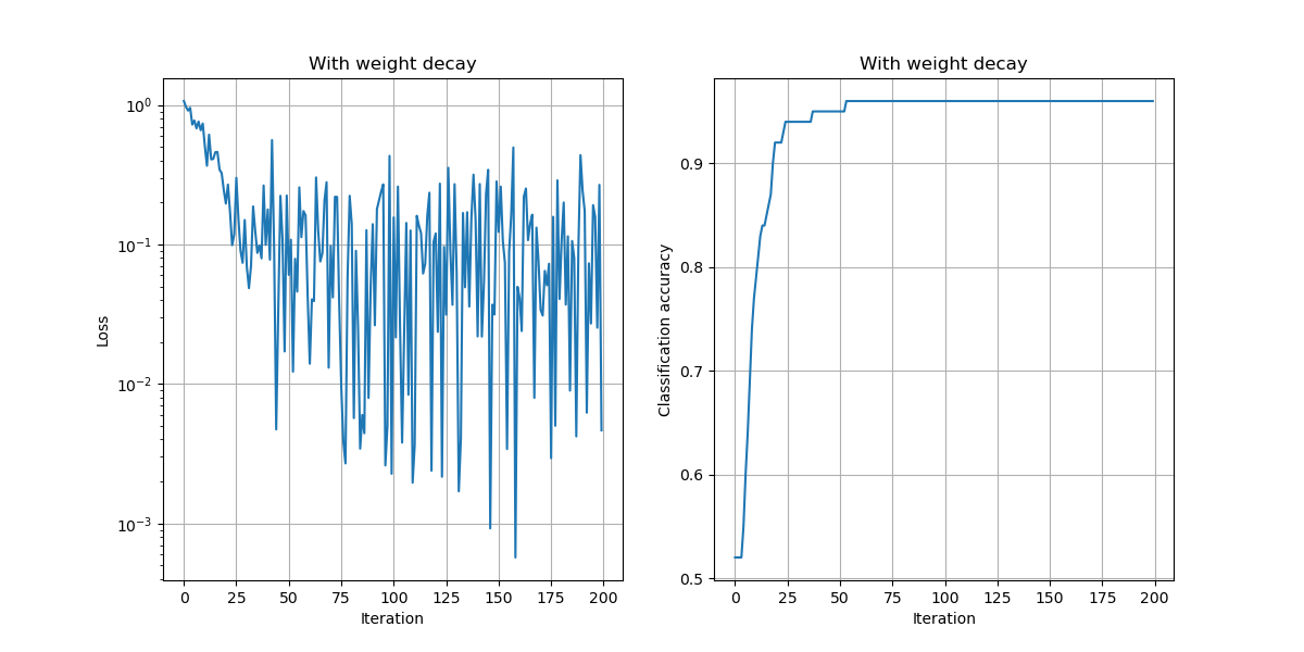
Now add weight decay and observe the changes to the training loss and accuracy.
Setting:
Observations:
# Part b)
# loss function and optimizer
criterion = nn.BCELoss(reduction='mean') # binary cross-entropy loss, use mean loss
lr = 1e-2 # learning rate

# no weight decay
plot_probs = True
logreg_model = LogisticRegression(2)
optimizer = torch.optim.SGD(logreg_model.parameters(), lr=lr, momentum=0.99)
# training loop
n_iter = 200
batch_size = 16
loss_values, accuracies = [], []
for n in range(n_iter):
    # zero out gradients
    optimizer.zero_grad()
    # sample random batch and pass to model
    batch_indices = np.random.choice(np.arange(len(labels)), size=batch_size)
    input_batch = input_data[batch_indices].unsqueeze(-1) # make dimensions match for matrix multiplication
    label_batch = labels[batch_indices]
    predictions = logreg_model(input_batch).squeeze(-1) # make dimensions match for loss function
    # calculate loss
    loss = criterion(predictions, label_batch)
    # backpropagate and update
    loss.backward()
    optimizer.step()
    # logging
    loss_values.append(loss.item())
    accuracies.append(model_accuracy(logreg_model, input_data, labels))
# plot model probabilities
if plot_probs:
    plot_model_probs(logreg_model, plus_class, negative_class)
    plt.savefig("./img/classification_no_weightdecay.png")
# plot loss values
plt.figure(figsize=(12,6))
plt.subplot(121)
plt.semilogy(loss_values)
plt.grid(True)
plt.title('Without weight decay')
plt.xlabel('Iteration')
plt.ylabel('Loss')
plt.subplot(122)
plt.plot(accuracies)
plt.grid(True)
plt.title('Without weight decay')
plt.xlabel('Iteration')
plt.ylabel('Classification accuracy')
plt.savefig("./img/lossacc_no_weightdecay.png")

# with weight decay
plot_probs = True
logreg_model = LogisticRegression(2) # re-initialize model
optimizer = torch.optim.SGD(logreg_model.parameters(), lr=lr, momentum=0.99, weight_decay=1e-2)
# training loop
n_iter = 200
batch_size = 16
loss_values, accuracies = [], []
for n in range(n_iter):
    # zero out gradients
    optimizer.zero_grad()
    # sample random batch and pass to model
    batch_indices = np.random.choice(np.arange(len(labels)), size=batch_size)
    input_batch = input_data[batch_indices].unsqueeze(-1) # make dimensions match for matrix multiplication
    label_batch = labels[batch_indices]
    predictions = logreg_model(input_batch).squeeze(-1) # make dimensions match for loss function
    # calculate loss
    loss = criterion(predictions, label_batch)
    # backpropagate and update
    loss.backward()
    optimizer.step()
    # logging
    loss_values.append(loss.item())
    accuracies.append(model_accuracy(logreg_model, input_data, labels))
# plot model probabilities
if plot_probs:
    plot_model_probs(logreg_model, plus_class, negative_class)
    plt.savefig("./img/classification_w_weightdecay.png")
# plot loss values
plt.figure(figsize=(12,6))
plt.subplot(121)
plt.semilogy(loss_values)
plt.grid(True)
plt.title('With weight decay')
plt.xlabel('Iteration')
plt.ylabel('Loss')
plt.subplot(122)
plt.plot(accuracies)
plt.grid(True)
plt.title('With weight decay')
plt.xlabel('Iteration')
plt.ylabel('Classification accuracy')
plt.savefig("./img/lossacc_w_weightdecay.png")


 |
 |
 |
 |
Setting (right):
Observations:
In the above example, we chose a learning rate of $\alpha=10^{-2}$, used no momentum, used no weight decay, and trained the model for 200 iterations.
a) Compare the results of training with and without momentum, keeping the learning rate and number of iterations fixed.
Setting:
# Part a)
# loss function and optimizer
criterion = nn.BCELoss(reduction='mean') # binary cross-entropy loss, use mean loss
lr = 1e-2 # learning rate

# without momentum
plot_probs = True
logreg_model = LogisticRegression(2)
optimizer = torch.optim.SGD(logreg_model.parameters(), lr=lr)
# training loop
n_iter = 200
batch_size = 16
loss_values, accuracies = [], []
for n in range(n_iter):
    # zero out gradients
    optimizer.zero_grad()
    # sample random batch and pass to model
    batch_indices = np.random.choice(np.arange(len(labels)), size=batch_size)
    input_batch = input_data[batch_indices].unsqueeze(-1) # make dimensions match for matrix multiplication
    label_batch = labels[batch_indices]
    predictions = logreg_model(input_batch).squeeze(-1) # make dimensions match for loss function
    # calculate loss
    loss = criterion(predictions, label_batch)
    # backpropagate and update
    loss.backward()
    optimizer.step()
    # logging
    loss_values.append(loss.item())
    accuracies.append(model_accuracy(logreg_model, input_data, labels))
# plot model probabilities
if plot_probs:
    plot_model_probs(logreg_model, plus_class, negative_class)
    plt.savefig("./img/classification_no_momentum.png")
# plot loss values
plt.figure(figsize=(12,6))
plt.subplot(121)
plt.semilogy(loss_values)
plt.grid(True)
plt.title('Without momentum')
plt.xlabel('Iteration')
plt.ylabel('Loss')
plt.subplot(122)
plt.plot(accuracies)
plt.grid(True)
plt.title('Without momentum')
plt.xlabel('Iteration')
plt.ylabel('Classification accuracy')
plt.savefig("./img/lossacc_no_momentum.png")


# with momentum
plot_probs = True
logreg_model = LogisticRegression(2) # re-initialize model
optimizer = torch.optim.SGD(logreg_model.parameters(), lr=lr, momentum=0.5)
# training loop
n_iter = 200
batch_size = 16
loss_values, accuracies = [], []
for n in range(n_iter):
    # zero out gradients
    optimizer.zero_grad()
    # sample random batch and pass to model
    batch_indices = np.random.choice(np.arange(len(labels)), size=batch_size)
    input_batch = input_data[batch_indices].unsqueeze(-1) # make dimensions match for matrix multiplication
    label_batch = labels[batch_indices]
    predictions = logreg_model(input_batch).squeeze(-1) # make dimensions match for loss function
    # calculate loss
    loss = criterion(predictions, label_batch)
    # backpropagate and update
    loss.backward()
    optimizer.step()
    # logging
    loss_values.append(loss.item())
    accuracies.append(model_accuracy(logreg_model, input_data, labels))
# plot model probabilities
if plot_probs:
    plot_model_probs(logreg_model, plus_class, negative_class)
    plt.savefig("./img/classification_w_momentum.png")
# plot loss values
plt.figure(figsize=(12,6))
plt.subplot(121)
plt.semilogy(loss_values)
plt.grid(True)
plt.title('With momentum')
plt.xlabel('Iteration')
plt.ylabel('Loss')
plt.subplot(122)
plt.plot(accuracies)
plt.grid(True)
plt.title('With momentum')
plt.xlabel('Iteration')
plt.ylabel('Classification accuracy')
plt.savefig("./img/lossacc_w_momentum.png")


|
|
|
|
Observations: