Lecture 13 - Midterm review

ECE364 - Programming Methods for Machine Learning

Nickvash Kani

Slides based off prior lectures by Alex Schwing, Aigou Han, Farzad Kamalabadi, Corey Snyder. All mistakes are my own!

In this lecture:

• Sample questions to prepare for the Midterm on Tuesday

import torch
import numpy as np

PyTorch basics, tensors, storage and memory, indexing and slicing, derivatives and chain rule

• Tensors are the primary class we use for storing and acting on data in PyTorch.
  • Choosing the appropriate data type and shape for a tensor is important to efficiently store data.
• Operations on tensors can either create a new tensor or create a view of a Tensor.
  • For example operations with an underscore, e.g. torch.cos_(x), operate in-place and thus do not allocate new memory.
• Tensor views share the same underlying memory and thus point to the same locations in memory.
• Tensor/array slicing are efficient ways to access or collect values according to certain conditions from a tensor/array
  • We may use slicing to extract only a particular column or every other element in a row, for example.
  • We may use Boolean operators to create truth arrays to separate elements based on a condition
• We also reviewed differentiation and chain rule as they play a core role to auto-differentiation engines like PyTorch

import torch
a = torch.zeros(3, 2)
b = a.cos_()
c = a+b

a) Does b share the same pointer as a?

def same_storage(x, y):
    return x.storage().data_ptr() == y.storage().data_ptr()

print(same_storage(a,b))

True

Does c share the same pointer as b?

print(same_storage(a,c))

False

b) What would be printed if we ran print(a, b, c)?

print("A: " + str(a) + "\n" + "B: " + str(b) + "\n" + "C: " + str(c))

A: tensor([[1., 1.],
        [1., 1.],
        [1., 1.]])
B: tensor([[1., 1.],
        [1., 1.],
        [1., 1.]])
C: tensor([[2., 2.],
        [2., 2.],
        [2., 2.]])

Slicing and truth arrays practice

Consider the below code snippet which creates a (10, 10) Tensor of random integers between $\{-99, 99\}$.

import torch
a = torch.randint(low=-99, high=100, size=(10, 10))
print(a)
#d = a[b, c]
#e = a[f, g]
#h = e[i]

tensor([[ 69, -57,  56, -57,  -7,  77, -87,  71,  -2, -83],
        [ 68,  98, -77,  -1,  66, -66,  41, -71,  24,  39],
        [-70,   2, -61, -60, -68,  41, -81, -22, -90, -58],
        [ 57,  78,  -1,  58, -50, -19, -64,  23,  75,  57],
        [-37,  51, -65,  87,  75,  66, -51,  -6,  88, -62],
        [-84,  -6,  50, -11, -11, -76, -76, -31,  97,  41],
        [ 86, -37, -47,  65,  -2, -45,  19,  35,  17, -19],
        [-27,  76,  42,  43,  65,  40,  83, -17, -26,  24],
        [-99,  69,  96, -78, -82, -86,  46, -19,  68,  74],
        [-72, -38,  -8, -67,   1, -55,  97, -76,   2, -38]])

a) We would like for d to contain the top-right quadrant of a. What should b and c be to accomplish this?

d = a[ 0:int(a.shape[0]/2), 5:10]
print(d)

tensor([[ 90,  34,  49,  55,  18],
        [ 64, -31, -41, -54,   3],
        [-50,  12, -41, -78, -77],
        [-13,  10, -76, -19,  58],
        [-71, -31, -53, -62,  83]])

print(a[0:int(a.shape[0]/2), 0:int(a.shape[1]/2)])

b) We would like for h to contain all multiples of 4 in column three of a. What should f, g and i be to accomplish this? Note: you may assume the "zeroth" column refers to index 0, "first" to index 1, and so on.

e = a[:, 3]
i = e%4==0
h = e[i]
#h=[]
#for i in range(len(e)): 
#    if e[i] % 4 == 0: 
#        h.append(e[i])
print(e)

tensor([-57,  -1, -60,  58,  87, -11,  65,  43, -78, -67])

e = a[:,3]
h = e[e%4==0]
print(h)

Linear algebra review, linear algebra with PyTorch, more differentiation and chain rule including matrices and vectors

• We reviewed linear algebra basics including dot products, matrix operations: multiplication, element-wise product, transpose, inverse, norms, gradients, and basic eigendecomposition.
• PyTorch readily performs linear algebra operations and may help us automate common calculations like solving systems of equations (via matrix inverse), for example.
• Multivariable functions have partial deriviatives with respect to each function variable. The collection of partial derivatives is referred to as the gradient.
• Scalar or vector-valued functions with vector and matrix arguments may also have partial derivatives with respect to the scalar or matrix arguments.
• For vector-valued functions, we have the Jacobian which represents the partial derivative of each entry in the output vector with repect to each element in the input vector.
• Scalar-valued example (gradient): $x\in\mathbb{R}^n,~y\in\mathbb{R}^n, A\in\mathbb{R}^{n\times n}$

$$ f(x, y, A) = y^\top Ax \in\mathbb{R}. $$$$ \frac{\partial f}{\partial x} = \begin{bmatrix}\frac{\partial f}{\partial x_1} & \frac{\partial f}{\partial x_2} & \cdots \frac{\partial f}{\partial x_n} \end{bmatrix}^{\top} $$

Note that the shape of $\frac{\partial f}{\partial x}$ matches the shape of $x$!

• Vector-valued example (Jacobian): $x\in\mathbb{R}^n, A\in\mathbb{R}^{m\times n}$

$$ \mathbf{f}(x, A) = Ax \in\mathbb{R}^{m} $$$$ \frac{\partial \mathbf{f}}{\partial x} = \begin{bmatrix} \frac{\partial f_1}{\partial x_1} & \frac{\partial f_1}{\partial x_2} & \cdots & \frac{\partial f_1}{\partial x_n}\\ \frac{\partial f_2}{\partial x_1} & \frac{\partial f_2}{\partial x_2} & \cdots & \frac{\partial f_2}{\partial x_n}\\ \vdots & \vdots & \vdots & \vdots\\ \frac{\partial f_m}{\partial x_1} & \frac{\partial f_m}{\partial x_2} & \cdots & \frac{\partial f_m}{\partial x_n}\\ \end{bmatrix}\in\mathbb{R}^{m\times n} $$

Sample problem

Assume $x\in\mathbb{R}^n$ and $A\in\mathbb{R}^{m\times n}$.

Compute $\frac{\partial f}{\partial x}$ for $f(x) = \frac{1}{2}\lVert Ax\rVert_2^2$.

We may approach the partial $\frac{\partial f}{\partial x}$ in a couple different ways.

Option 1:

Let $y=Ax$. We may then write $$ \begin{align*} \frac{1}{2}\lVert Ax\rVert_2^2 &= \frac{1}{2}\lVert y\rVert_2^2\\ \frac{\partial f}{\partial x} &= \frac{\partial f}{\partial y}\frac{\partial y}{\partial x}. \end{align*} $$ Above, we use chain rule to re-write the desired partial derivative where $\frac{\partial y}{\partial x}\in\mathbb{R}^{m\times n}$ is the Jacobian of $y$ with respect to $x$. Let $J_y\in \mathbb{R}^{m\times n}$ be this Jacobian $\frac{\partial y}{\partial x}$. In matrix form, $J_y$ will look like $$ J_y = \begin{bmatrix} \frac{\partial y_1}{\partial x_1} & \frac{\partial y_1}{\partial x_2} & \cdots & \frac{\partial y_1}{\partial x_n}\\ \frac{\partial y_2}{\partial x_1} & \frac{\partial y_2}{\partial x_2} & \cdots & \frac{\partial y_2}{\partial x_n}\\ \vdots & \vdots & \ddots & \vdots\\ \frac{\partial y_m}{\partial x_1} & \frac{\partial y_m}{\partial x_2} & \cdots & \frac{\partial y_m}{\partial x_n} \end{bmatrix}. $$ The partial derivative $\frac{\partial f}{\partial y}$ will be a vector in $\mathbb{R}^{m}$. Thus, we have two ways to express express $\frac{\partial f}{\partial x}$: $$ \begin{align*} \frac{\partial f}{\partial x} &= J_y^\top\frac{\partial f}{\partial y} = \begin{bmatrix} \frac{\partial y_1}{\partial x_1} & \frac{\partial y_2}{\partial x_1} & \cdots & \frac{\partial y_m}{\partial x_1}\\ \frac{\partial y_1}{\partial x_2} & \frac{\partial y_2}{\partial x_2} & \cdots & \frac{\partial y_m}{\partial x_2}\\ \vdots & \vdots & \ddots & \vdots\\ \frac{\partial y_1}{\partial x_n} & \frac{\partial y_m}{\partial x_2} & \cdots & \frac{\partial y_m}{\partial x_n} \end{bmatrix}\begin{bmatrix} \frac{\partial f}{\partial y_1}\\ \frac{\partial f}{\partial y_2}\\ \vdots\\ \frac{\partial f}{\partial y_m} \end{bmatrix}\\ \frac{\partial f}{\partial x} &= \left(\frac{\partial f}{\partial y}\right)^\top J_y = \begin{bmatrix} \frac{\partial f}{\partial y_1} & \frac{\partial f}{\partial y_2} & \cdots & \frac{\partial f}{\partial y_m} \end{bmatrix}\begin{bmatrix} \frac{\partial y_1}{\partial x_1} & \frac{\partial y_1}{\partial x_2} & \cdots & \frac{\partial y_1}{\partial x_n}\\ \frac{\partial y_2}{\partial x_1} & \frac{\partial y_2}{\partial x_2} & \cdots & \frac{\partial y_2}{\partial x_n}\\ \vdots & \vdots & \ddots & \vdots\\ \frac{\partial y_m}{\partial x_1} & \frac{\partial y_m}{\partial x_2} & \cdots & \frac{\partial y_m}{\partial x_n} \end{bmatrix} \end{align*} $$ The first solution would give us $\frac{\partial f}{\partial x}\in\mathbb{R}^n$ while the second solution is the transpose of this with $\frac{\partial f}{\partial x}\in\mathbb{R}^{1\times n}$.

With the application of chain rule set, we may determine the require partial derivatives and obtain the solution. $$ \begin{align*} f(y) &= \frac{1}{2}\lVert y\rVert_2^2\\ &= \frac{1}{2}y^\top y\\ \frac{\partial f}{\partial y} &= y \end{align*} $$ To find the Jacobian $J_y$, it is helpful to consider the partial derivative of one element in $y$ with respect to $x$. Let $a_i^\top$ represent the $i$'th row in $A$. Thus, $y_i=a_i^\top x$. Therefore, $\frac{\partial y_i}{\partial x}$, which is the $i$'th row in $J_y$ will be $a_i^\top$. In other words, the rows of $A$ become the rows of $J_y$. Therefore, $J_y=A$. Plugging these results into our expression of chain rule, we find \begin{align*} \frac{\partial f}{\partial x} &= J_y^\top\frac{\partial f}{\partial y}\\ &= A^\top y\\ &= A^\top Ax. \end{align*} It is important to note that the Jacobian is defined as being $m\times n$ for functions mapping from $\mathbb{R}^n$ to $\mathbb{R}^m$ like in the above example. However, we had to consider transposing the Jacobian and left-multiplying to make sure chain rule was carried out correctly like in the $J_y^\top y$ equations above. Notice how the matrix-vector multiplication accumulates the partial derivatives of each $x_i$ from each $y_j$

Option 2

The alternative we may examine involves expanding the L2 norm and using the product rule of differentation. $$ \begin{align*} f(x) &= \frac{1}{2}\lVert Ax\rVert_2^2\\ &= \frac{1}{2}(Ax)^\top(Ax)\\ \end{align*} $$ Computing the partial derivative: $$ \begin{align*} \frac{\partial f}{\partial x} &= \frac{1}{2}\left(\frac{\partial (Ax)^\top}{\partial x}Ax+(Ax)^\top\frac{\partial (Ax)}{\partial x}\right)\\ &= \frac{1}{2}\left(\left(\frac{\partial Ax}{\partial x}\right)^\top Ax+\left(\frac{\partial Ax}{\partial x}\right)^\top Ax\right)\\ &= \frac{1}{2}\left(\frac{\partial (Ax)^\top}{\partial x}Ax+\left(\frac{\partial (Ax)^\top}{\partial x}\right) Ax\right)\\ &= \frac{\partial (Ax)^\top}{\partial x}Ax\\ &= A^\top Ax. \end{align*} $$ Above, note that we re-distribute the transpose in the second term in the second line so that we may combine like terms, i.e. $(CD)^\top=D^\top C^\top$ where we have $C=(Ax)^\top$ and $D=\frac{\partial Ax}{\partial x}$. In the last line, we borrow our result from Option 1 where $\frac{\partial Ax}{\partial x}=A$ and thus $\frac{\partial (Ax)^\top}{\partial x}=A^\top$.

Gradient descent, computational graphs, backpropagation

• Derivatives and gradients are critical to minimizing or maximizing functions. Function optimization is at the heart of machine learning and data science problems where we seek to minimize a cost function or maximize or a reward function by learning from data.
• Most functions and real-world problems cannot be optimized in closed-form by solving for where the derivative is equal to zero. This motivates the use of gradient-based methods like gradient descent.
• Gradient descent is an iterative algorithm that updates parameters by stepping in the direction of the negative gradient (direction of steepest descent).
• The gradient descent equation for function $f(x)$ at iteration $k+1$ is stated as

$$ x^{(k+1)} = x^{(k)}-\alpha\nabla f(x) $$

where $\alpha$ is the step-size or learning rate to control the size of each update step.

• Auto-differentiation engines operate based on computational graphs that build up complicated functions from simple mathematical operations using directed acyclic graphs. These graphs give important structure for computation.
• Performing gradient descent by hand is intractable for larger or more complicated functions even if we may determine the derivatives using chain rule. Thus, we would like to automate computing gradients. Methods like numeric differentiation or symbolic differentation are possible, however, we focus on auto-differentiation via backpropagation as the most scalable method for machine learning.
• Backpropagation works in two stages: (1) forward pass and (2) backward pass.
  • Forward pass: inputs are passed to the computational graph and intermediate values are stored at each node of computation of the graph
  • Backward pass: well-defined gradient functions at each node utilize the values from forward propagation to transmit partial derivatives to each predecessor node. The adjoint, partial derivative with respect to each seed node, at each node is composed of the adjoints of all successors and the partial derivatives of each successor with respect to the current node:

$$ \bar{w}_i = \sum_{j\in\textrm{successors}(i)}\bar{w}_j\frac{\partial w_j}{\partial w_i}. $$ The above equation demonstrates chain rule!

Backpropagation practice

Consider the following multivariable function $$ f(x, y) = 2\cos^2(xy)+\ln(\cos(xy)) $$

a) Determine each partial derivative $\frac{\partial f}{\partial x}$, $\frac{\partial f}{\partial y}$.

The below computational graph depicts $f(x, y)$.

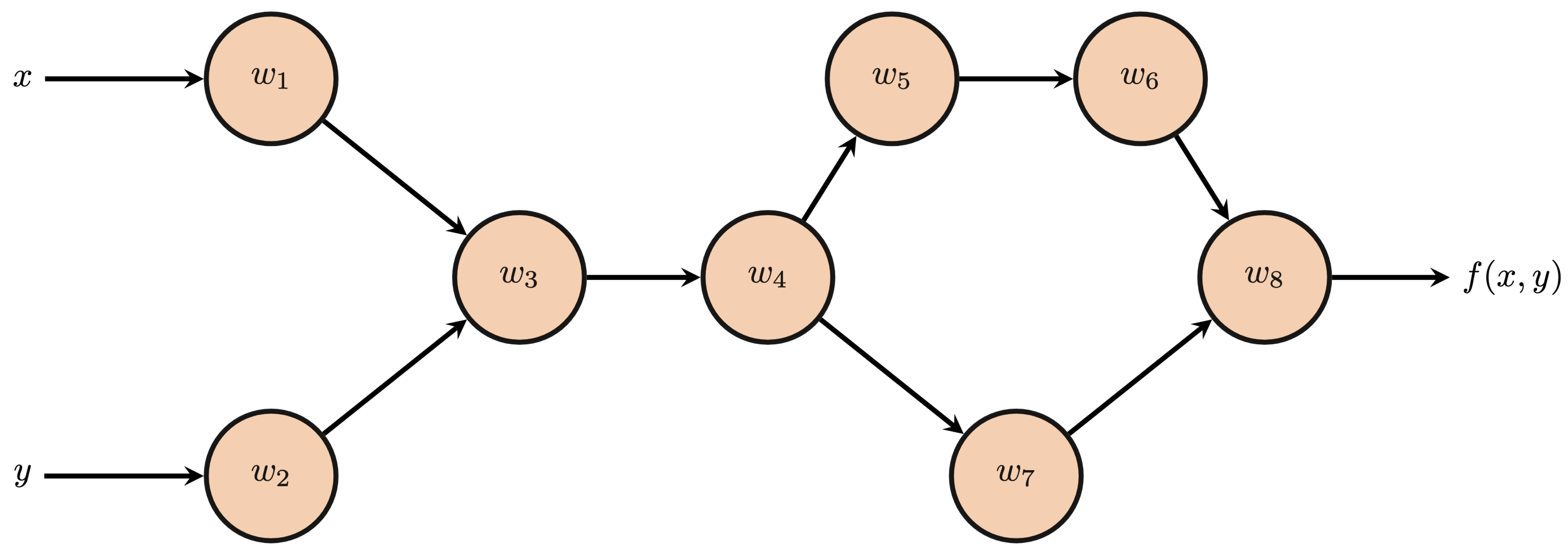
b) Determine the values of each node $w_i$

c) Determine the partial derivatives for each successor node with respect to its predecessor nodes.

d) Compute the adjoints of all nodes. Verify that your expressions for $\bar{w}_1$ and $\bar{w}_2$ match your partial derivatives from part (a).

Backpropagation practice

Consider the following multivariable function $$ f(x, y) = 2\cos^2(xy)+\ln(\cos(xy)) $$

a) Determine each partial derivative $\frac{\partial f}{\partial x}$, $\frac{\partial f}{\partial y}$.

$$ \begin{align*} \frac{\partial f}{\partial x} &= -4y\cos(xy)\sin(xy)-\frac{y\sin(xy)}{\cos(xy)}\\ \frac{\partial f}{\partial y} &= -4x\cos(xy)\sin(xy)-\frac{x\sin(xy)}{\cos(xy)} \end{align*} $$

The below computational graph depicts $f(x, y)$.

b) Determine the values of each node $w_i$ $$ \begin{align*} w_1 &= x &w_2&=y\\ w_3 &=w_1w_2 &w_4&= \cos(w_3)\\ w_5 &= w_4^2 &w_6&=2w_5\\ w_7 &= \ln(w_4) &w_8&=w_6+w_7 \end{align*} $$

c) Determine the partial derivatives for each successor node with respect to its predecessor nodes. $$ \begin{align*} \frac{\partial w_8}{\partial w_7} &= 1 &\frac{\partial w_8}{\partial w_6} &= 1\\ \frac{\partial w_7}{\partial w_4} &= \frac{1}{w_4} &\frac{\partial w_6}{\partial w_5} &= 2\\ \frac{\partial w_5}{\partial w_4} &= 2w_4 &\frac{\partial w_4}{\partial w_3} &= -\sin(w_3)\\ \frac{\partial w_3}{\partial w_2} &= w_1 &\frac{\partial w_3}{\partial w_1} &= w_2\\ \end{align*} $$

d) Compute the adjoints of all nodes. Verify that your expressions for $\bar{w}_1$ and $\bar{w}_2$ match your partial derivatives from part (a). $$ \begin{align*} \bar{w}_8 &= 1 &\bar{w}_7&=1\\ \bar{w}_6 &= 1 &\bar{w}_5&=2\\ \bar{w}_4 &= \frac{1}{w_4} + 4w_4 &\bar{w}_3&= -\frac{\sin(w_3)}{w_4} -4w_4\sin(w_3)\\ \bar{w}_2 &= -\frac{w_1\sin(w_3)}{w_4} -4w_1w_4\sin(w_3) &\bar{w}_1 &= -\frac{w_2\sin(w_3)}{w_4} -4w_2w_4\sin(w_3) \end{align*} $$ Recursively plugging in using the expressions from part (b): $$ \begin{align*} \bar{w}_1 &= \frac{\partial f}{\partial w_1} = -4y\cos(xy)\sin(xy)-\frac{y\sin(xy)}{\cos(xy)} \\ \bar{w}_2 &= \frac{\partial f}{\partial w_2} = -4x\cos(xy)\sin(xy)-\frac{x\sin(xy)}{\cos(xy)} \end{align*} $$

Linear regression: one-dimensional, multi-dimensional, transformations of inputs

• Linear regression in one dimension seeks to find a line-of-best-fit for a dataset of $(x, y)$ coordinates.
• Consider $\mathcal{D}=\{(x_i, t_i)\}_{i=1}^{N}$. Linear regression minimizes:

$$ \min_{w_1,~w_0}~\frac{1}{2}\sum_{i=1}^{N}(t_i-w_1x_i-w_0)^2, $$

where $w_0$ represents the bias term, i.e. y-intercept.

• This may also be written in vector form:

$$ \min_{w}~\frac{1}{2}\lVert \mathbf{X}^\top w - t\rVert_2^2, $$

where $$ \mathbf{X}^\top = \begin{bmatrix} x_1 & 1\\ x_2 & 1\\ \vdots & \vdots \\ x_N & 1 \end{bmatrix} $$

• By taking the gradient of the objective functions and setting to zero, we may obtain a closed-form solution for linear regression

$$ w^*=(\mathbf{X}\mathbf{X}^\top)^{-1}\mathbf{X}t. $$

• We may also have linear regression in higher dimensions, e.g. plane-of-best-fit, hyperplane-of-best-fit.
• Alternatively, linear regression may be applied to more complicated regression problems where transformations are applied to input variables, e.g. polynomial regression like third-order polynomial regression below.

$$ \min_{w_3,~w_2,~w_1,~w_0}~\frac{1}{2}\sum_{i=1}^{N}(t_i-w_3x_i^3-w_2x_i^2-w_1x_i-w_0)^2 $$

• Where a transformation $\Phi(\mathbf{X})$ is applied to input data for linear regression, we may now describe the closed-form solution as

$$ w^*=(\mathbf{\Phi}\mathbf{\Phi}^\top)^{-1}\mathbf{\Phi}t. $$

• What happens if $\mathbf{X}^\top\in\mathbb{R}^{N\times d}$ has $d>N$?

Linear classification: linear classification and support vector machines

We introduced the concept of binary linear classifiers with simple threshold wrapper functions:

Binary linear classification

• classification: predict a discrete-valued target
• binary: predict a binary target $t \in \{0,1\}$
  • Training examples with $t = 1$ are called positive examples, and training examples with $t = 0$ are called negative examples.
• linear: model is a linear function of x, followed by a threshold:

$$ z = \mathbf{w}^T \mathbf{x} + b $$$$ y = \begin{cases} 1 & \text{if } z \geq r \\ 0 & \text{if } z < r \end{cases} $$

which reduces to:

$$ z = \mathbf{w}^T \mathbf{x} $$$$ y = \begin{cases} 1 & \text{if } z \geq 0 \\ 0 & \text{if } z < 0 \end{cases} =H(z) $$

But these models had the issue of penalizing over-confident predictions. A way to solve this issue was to build support-vector-machine models where data point within a pair of support vectors (margins) would be the only things to effect the training of the boundary. The binary cross entropy loss of a support vector machien was derived as:

$$ \mathcal{L} = \frac{\vert W[1:] \vert}{2} + C\sum \max\left( 0, t^{(i)} \cdot W x^{(i)} \right)^2 $$

where the left term maximizes the margin and the right term fits the boundary. The parameter C controls how much focus the optimizer puts toward each goal.

Logistic Regression

Logistic regression as was another classification model that is trainable by backpropagation. For an input vector $x\in\mathbb{R}^N$, logistic fits a parameter vector $w\in\mathbb{R}^N$ and a bias term $b\in\mathbb{R}$ to perform the binary classification problem where labels $y\in\{-1, +1\}$. The logistic regression function $f_\theta(x)$ can be seen as fitting a sigmoid function around a linear regression model:

$$ f_\theta(x) = \mathbf{Pr}\{Y=1|x\}=\frac{1}{1+e^{-(w^\top x + b)}}. $$

Above, if the regression score $z= w\top x+b$ is a larger positive number, the probability of the positive class, i.e. label $+1$, approaches 1. Conversely, if this regression score is small, i.e. very negative, the probability of the positive class will approach 0 as the probability of the negative class, i.e. label $-1$, approaches 1. To train a logistic regression model, we are minimizing the negative log likelihood (similarly, maximizing the log likelihood) of the available labels for the given data in order to learn the parameters $\theta=\{w, b\}\in\mathbb{R}^{N+1}$. With respect to a PyTorch implementation, this means we will use binary cross-entropy loss function.

Recall that we can also define a multi-class logistic regression model as performing a matrix-vector multiplication with an input vector $x\in\mathbb{R}^N$ to produce class scores $z\in\mathbb{R}^M$.

$$ \begin{align} z &= Wx+b\\ &= \begin{bmatrix} \rule[.6ex]{4ex}{0.75pt} & w_1^\top & \rule[.6ex]{4ex}{0.75pt}\\ \rule[.6ex]{4ex}{0.75pt} & w_2^\top & \rule[.6ex]{4ex}{0.75pt}\\ & \vdots & \\ \rule[.6ex]{4ex}{0.75pt} & w_M^\top & \rule[.6ex]{4ex}{0.75pt}\\ \end{bmatrix}\begin{bmatrix} \rule[-1ex]{0.5pt}{4ex}\\ x\\ \rule[1ex]{0.5pt}{4ex}\\ \end{bmatrix} +\begin{bmatrix} b_1\\ b_2\\ \vdots\\ b_M \end{bmatrix}\\ &= \begin{bmatrix} z_1\\ z_2\\ \vdots\\ z_M \end{bmatrix} \end{align} $$

The resulting class scores are then converted to class probabilities using the softmax function.

$$ \textrm{softmax}(z)_k=\mathbf{Pr}\{\textrm{Class }y=k|x\} = \frac{e^{z_k}}{\sum_{j=1}^{M}e^{z_j}}. $$

Instead of binary cross-entropy, we will instead now use cross-entropy loss. For label $y_i\in\{1, \ldots, M\}$, we compute cross-entropy loss across dataset $\mathcal{D}={(x_i, y_i)}_{i=1}^{N}:

$$ \ell_{\textrm{ce}} = -\sum_{i=1}^{N}\log\left(f_{y_i}(x_i; \theta)\right), $$

where $f_{y_i}(x_i; \theta)$ computes the probability of class $y_i$ given input $x_i$ according to the softmax outputs of the multi-class logistic regression model.

PyTorch nn.Modules, Optimizers, Datasets, Dataloaders

nn.Modules

The nn.Module class is the universal base class for neural networks, and more broadly trainable models, in PyTorch found within the torch.nn package, i.e. torch.nn.Module. We create our own models by inheriting this base class and implementing the necessary methods for the class. There are two methods which must be implemented: __init__ and forward.

The __init__ method specifies the constructor and thus how every instance of this module must be initialized the __init__ method must first call super().__init__() to call the constructor of the base nn.Module class (and thus access all the helpful attributes and methods within). The forward method implements how the model processes input data for its forward pass.

The nn.Module base class also implements a highly useful functionality. Recall from our backpropagation lectures how we had to manually collect all of the trainable parameters to perform gradient descent, i.e. specify the update and clearing the gradients for each one. The nn.Module class automatically collects all learnable paramters in the .parameters() attribute. This makes scaling our models and learning algorithms dramatically easier!

Optimizers

The torch.optim package contains many helpful optimizers, i.e. learning algorithms, and other useful interfaces to simplify the parameter updating process. The simplest optimizer in the torch.optim package is the optim.SGD, which implements stochastic gradient descent (SGD). Also known as mini-batch gradient descent, SGD implements gradient descent except only computes the gradient over a random subset, or mini-batch, of the data. Thus, the computed gradient depends on a stochastic sample of the dataset. If the batch size for SGD is the entire dataset, then SGD simply becomes ordinary gradient descent.

Pros:

• Faster than gradient descent
• Noisier gradients from random subsets can help exit local minima

Cons:

• Can have slower convergence due to noisy gradients

Dataset Class

PyTorch offers an abstract base class for creating datasets that simplifies the process of building, manipulating, and sampling datasets, e.g. into training, validation, and testing sets. The torch.utils.data.Dataset class requires any new class that inherits this base class to implement three methods:

• __init__: The __init__ method is the constructor for the new dataset. Unlike the nn.Module class, the base class constructor does not need to be called, i.e. we do not need to call super().__init__(). The constructor is most commonly used to establish the data for the dataset or the necessary information to assign attributes that will assist the data retrieval process in the __getitem__ method.

• __len__: The __len__ method overrides the len() function in Python to determine the length of the dataset. In other words, for a dataset named my_dataset. The implemented __len__ function will allow len(my_dataset) to return the length of the dataset.

• __getitem__: The __getitem__ method overloads the use of brackets to index items in a dataset. For example, a dataset named my_dataset will call the __getitem__ method when we use my_dataset[i] and the index i is an input to the __getitem__ method.

With a PyTorch Dataset class in hand, we may take advantage of the torch.utils.data.DataLoader interface that will simplify the process of sampling batches of data; shuffling the dataset; partitioning into training set, validation set, testing set; and more! A DataLoader does not need to be implemented like a Dataset or nn.Module class. Instead, we only need to provide a Dataset object as input alongside several optional inputs:

• batch_size: number of examples in each batch or call to the dataloader

• shuffle: Boolean option to shuffle dataset each pass or epoch through the dataset

• sampler: Sampler object that specifies how data will be extracted from the dataset. For example, the SubsetRandomSampler allows us to specify indices within the larger dataset to sample at random. This is an easy way to create training, validation, and testing sets!

PyTorch training loop

Finally, we have all the necessary ingredients to create a PyTorch training loop! This training loop, while basic, forms the core of any model training code within PyTorch. Before executing the training loop, we need to ensure a few things are set:

• The model is instantiated/initialized.
• The dataset is prepared.
• The loss function and optimizer are instantiated.

With these in hand, the training loop takes on the following basic cycle for optimizer named optimizer and loss function named criterion:

1. Zero out the gradients using the optimizer using optimizer.zero_grad().
2. Pass the current batch or entire dataset to the model to generate predictions.
3. Calculate loss from criterion.
4. Backpropagate from loss value and perform gradient descent update by optimizer.step()
5. (Optional) Perform any desired logging, e.g. loss values, performance metrics, etc.

Best thing to do is look at a sample that incorporates the torch.nn model and Dataset classes:

# code from previous lecture
import numpy as np
import matplotlib.pyplot as plt
import torch
import torch.nn as nn
from torch.utils.data import Dataset
from torch.utils.data import DataLoader
from torch.utils.data import SubsetRandomSampler

class LogisticRegression(nn.Module):
    def __init__(self, N):
        super().__init__()
        self.w = nn.Parameter(torch.ones(N))
        self.b = nn.Parameter(torch.zeros(1))

    def forward(self, x):
        return 1/(1+torch.exp(-(self.w@x+self.b)))

class TwoClassDataset(Dataset):
    # don't forget the self identifier!
    def __init__(self, N, sigma):
        self.N = N # number of data points per class
        self.sigma = sigma # standard deviation of each class cluster
        self.plus_class = self.sigma*torch.randn(N, 2) + torch.tensor([-1, 1])
        self.negative_class = self.sigma*torch.randn(N, 2) + torch.tensor([1, -1])
        self.data = torch.cat((self.plus_class, self.negative_class), dim=0)
        self.labels = torch.cat((torch.ones(self.N), torch.zeros(self.N)))

    def __len__(self):
        return len(self.labels)

    def __getitem__(self, idx):
        x = self.data[idx]
        y = self.labels[idx]
        return x, y # return input and output pair
        
    
# compute classification accuracy
def model_accuracy(model, input_data, labels):
    predictions = model(input_data.unsqueeze(-1)).squeeze(-1)
    positive_preds = predictions >= 0.5
    negative_preds = predictions < 0.5
    n_correct = torch.sum(positive_preds*labels)+torch.sum(negative_preds*(1-labels))
    return n_correct

N = 100
sigma = 1.5
dataset = TwoClassDataset(N, sigma)
plus_data = dataset.plus_class
negative_data = dataset.negative_class

# create indices for each split of dataset
N_train = 60
N_val = 20
N_test = 20
indices = np.arange(len(dataset))
np.random.shuffle(indices)
train_indices = indices[:N_train]
val_indices = indices[N_train:N_train+N_val]
test_indices = indices[N_train+N_val:]

# create dataloader for each split
batch_size = 8
train_loader = DataLoader(dataset, batch_size=batch_size, sampler=SubsetRandomSampler(train_indices))
val_loader = DataLoader(dataset, batch_size=batch_size, sampler=SubsetRandomSampler(val_indices))
test_loader = DataLoader(dataset, batch_size=batch_size, sampler=SubsetRandomSampler(test_indices))

# training setup
criterion = nn.BCELoss(reduction='mean') # binary cross-entropy loss, use mean loss
lr = 1e-2 # learning rate
logreg_model = LogisticRegression(2) # initialize model
optimizer = torch.optim.SGD(logreg_model.parameters(), lr=lr, momentum=0.99, weight_decay=1e-3) # initialize optimizer

n_epoch = 100 # number of passes through the training dataset
loss_values, train_accuracies, val_accuracies = [], [], []
for n in range(n_epoch):
    epoch_loss, epoch_acc = 0, 0
    for x_batch, y_batch in train_loader:
        # zero out gradients
        optimizer.zero_grad()
        # pass batch to model
        predictions = logreg_model(x_batch.unsqueeze(-1)).squeeze(-1) # make dimensions match for loss function
        # calculate loss
        loss = criterion(predictions, y_batch)
        # backpropagate and update
        loss.backward()
        optimizer.step()
        # logging
        epoch_loss += loss.item()
        epoch_acc += model_accuracy(logreg_model, x_batch, y_batch)
    loss_values.append(epoch_loss/len(train_loader))
    train_accuracies.append(epoch_acc/N_train)
    # validation performance
    val_acc = 0
    for x_batch, y_batch in val_loader:
        # don't compute gradients since we are only evaluating the model
        with torch.no_grad():
            val_acc += model_accuracy(logreg_model, x_batch, y_batch)
    val_accuracies.append(val_acc/N_val)

plt.figure(figsize=(12,6))
plt.subplot(131)
plt.semilogy(loss_values)
plt.grid(True)
plt.title('Loss values')
plt.xlabel('Epoch')
plt.subplot(132)
plt.plot(train_accuracies)
plt.grid(True)
plt.title('Training Accuracy')
plt.xlabel('Epoch')
plt.subplot(133)
plt.plot(val_accuracies)
plt.grid(True)
plt.title('Validation Accuracy')
plt.xlabel('Epoch')

That's it for today

That's a breif overview of what we've learned. Remember, anything that has been in the lectures or homeworks is fair game. So review the lectures and hoemworks and I'll see you Tuesday!