In this lecture:
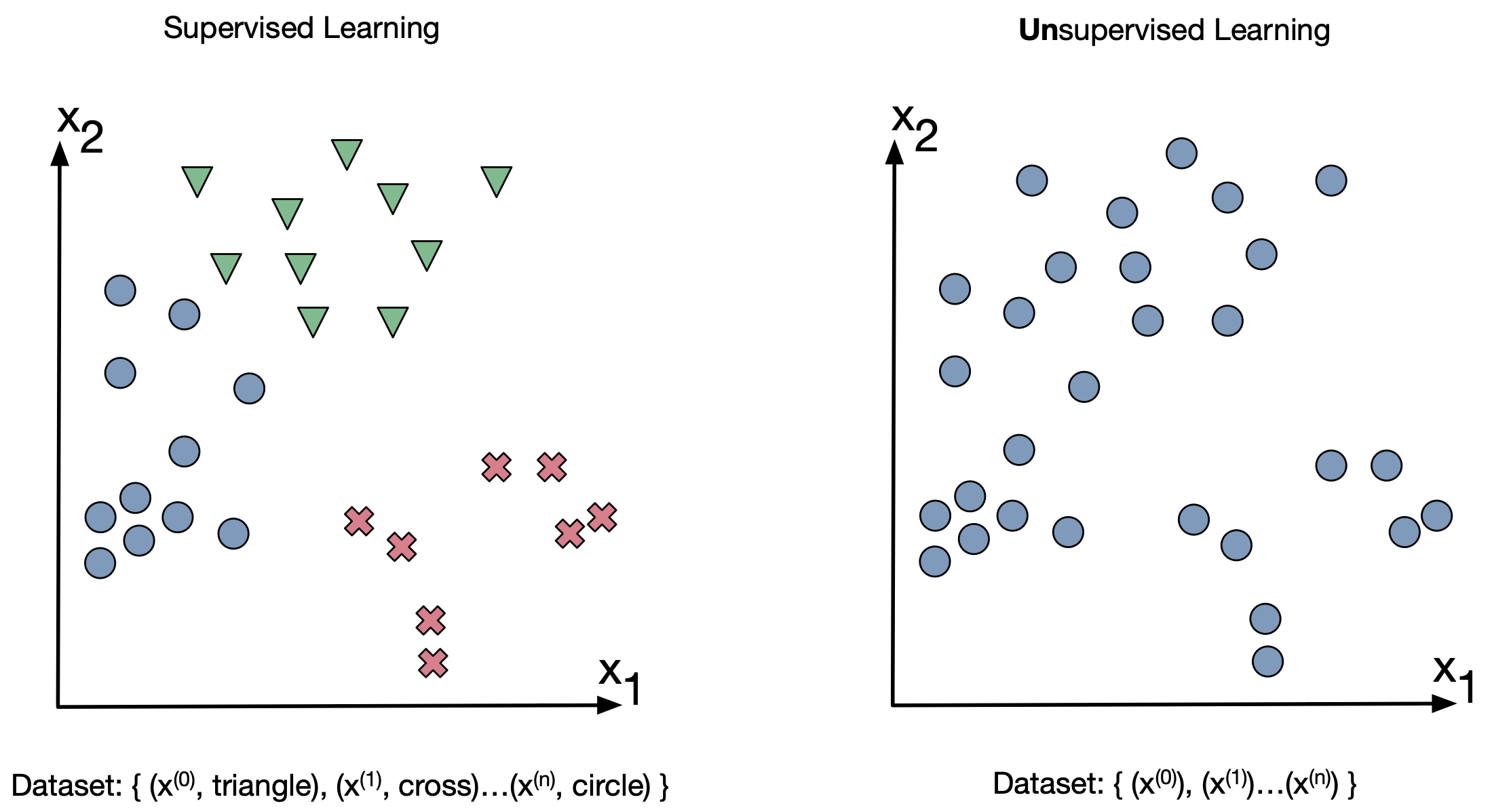
So far we've discussed supervised learning whihc is learning when there are labels attached to a input.
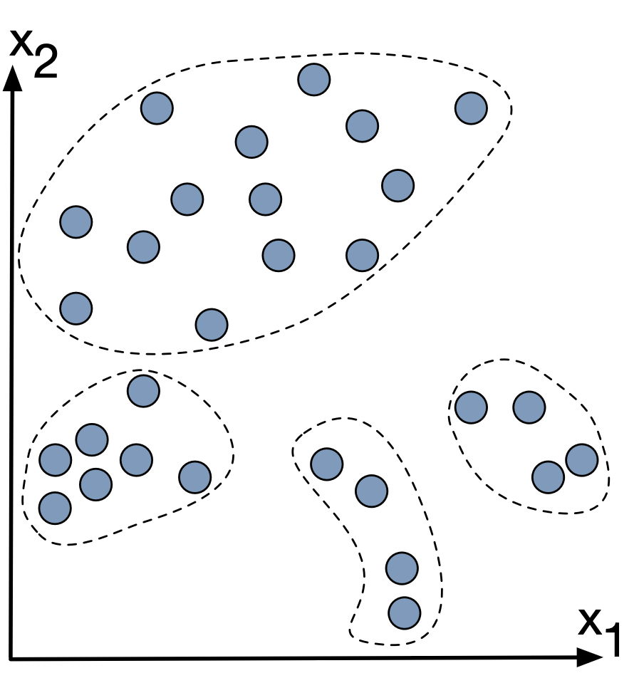
Unsupervised learning is when the data has no labels attached.
*Gratitude to Herman Kempar's excellent lectures on this topic
First we have to determine the number of clusters we want to partition the data into. Let's say there's $k$ clusters.
Starting work: for each datapoint, randomly assign it to one of $k$ clusters.
For each iteration:
for each cluster $k = 1 \rightarrow K$
for each data point $n = 1 \rightarrow N$
End when the data assignments to each cluster stop beign updated.
import numpy as np
import matplotlib.pyplot as plt
from sklearn.datasets import make_blobs

# 1. Generate synthetic data with 3 clusters, 20 points each

def generate_data(centers, k=3, n=20, seed=42):
    np.random.seed(seed)
    data = []
    for cx, cy in centers[:k]:
        cluster = np.random.randn(n, 2) + np.array([cx, cy])
        data.append(cluster)
    return np.vstack(data)

# 2. Randomly assign initial clusters
def initialize_clusters(data, k):
    return np.random.randint(0, k, size=len(data))

# 3. Calculate centroids based on current assignments
def calculate_centroids(data, assignments, k):
    centroids = np.array([data[assignments == i].mean(axis=0) if np.any(assignments == i) else np.random.randn(2) for i in range(k)])
    return centroids

# 4. Update assignments based on closest centroid
def update_assignments(data, centroids):
    distances = np.linalg.norm(data[:, np.newaxis] - centroids, axis=2)
    return np.argmin(distances, axis=1)

# 5. Plot data points and centroids
def plot_clusters(data, assignments, centroids):
    k = centroids.shape[0]
    colors = ['r', 'g', 'b', 'c', 'm', 'y']
    plt.figure(figsize=(6, 6))
    for i in range(k):
        points = data[assignments == i]
        plt.scatter(points[:, 0], points[:, 1], c=colors[i % len(colors)], label=f'Cluster {i}')
        plt.scatter(centroids[i, 0], centroids[i, 1], c=colors[i % len(colors)], marker='x', s=100, linewidths=3)
    plt.title("K-means Clustering")
    plt.legend()
    plt.grid(True)
    plt.show()
k=3
n=20
centers = [(0, 0), (5, 5), (0, 5)]
data = generate_data(n=n, k=k, centers=centers)
cluster_assignments = initialize_clusters(data, k)
centroids = calculate_centroids(data, cluster_assignments, k)
plot_clusters(data, cluster_assignments, centroids)

cluster_assignments = update_assignments(data, centroids)
plot_clusters(data, cluster_assignments, centroids)

centroids = calculate_centroids(data, cluster_assignments, k)
plot_clusters(data, cluster_assignments, centroids)

Notation:
for each cluster k = 1 to $K$: Calculate the cluster centroid $\mu_k$ as the mean of all the items assigned to cluster $k$
$\mu_k = \frac{1}{\vert C_k \vert} \Sigma_{i \in C_k} x^{\left(i\right)} $
for each item n = 1 to $N$: Assign item $x^{(n)}$ to the cluster with the closest centroid
$\text{arg}_k\text{min} \vert\vert x^{(n)} - \mu_k \vert\vert^2 $
For one cluster: Trying to optimize the distance between each of the items in a cluster to the centroid of the cluster.
$\Sigma_{i \in C_k} \vert\vert x^{(i)} - \mu_k \vert\vert^2 $
But we need to do this for every cluster:
$\Sigma^{K}_{k=1} \Sigma_{i \in C_k} \vert\vert x^{(i)} - \mu_k \vert\vert^2 $
but what is the loss a function of:
$J\left(C_1, \ldots, C_k, \mu_1, \ldots, \mu_k \right) = \Sigma^{K}_{k=1} \Sigma_{i \in C_k} \vert\vert x^{(i)} - \mu_k \vert\vert^2 $
k=3
n=20
centers = [(0, 0), (5, 5), (0, 1)]
data = generate_data(n=n, k=k, centers=centers, seed=1) #### try with seed 7 and seed 1
cluster_assignments = initialize_clusters(data, k)
centroids = calculate_centroids(data, cluster_assignments, k)

change_flag=True
num_iters=10
i = 0
while change_flag==True:
    change_flag=False
    i=i+1
    if i>num_iters:
        break
    cluster_assignments_new = update_assignments(data, centroids)
    assignments_differ = any(a != b for a,b in zip(cluster_assignments_new, cluster_assignments))
    if assignments_differ:
        change_flag = True
    cluster_assignments = cluster_assignments_new
    centroids = calculate_centroids(data, cluster_assignments, k)

plot_clusters(data, cluster_assignments, centroids)

K-means clustering is pretty good at distinguishing between clusters that are spacially dintinct.
But what if the clusters run into eachother?
Let's look at some data where K-means might not be the best option:
# -------------------------------------------------------------------------
# 1. Dataset Generation
# -------------------------------------------------------------------------

def generate_data(n_samples=300, random_state=42, plot_clusters=False, differentiated=True):
    """
    Generates a 2D dataset with two clusters.
    Both clusters overlap, providing a scenario where the GMM outperforms k-means.

    Optional plotting:
    - If 'plot_clusters' is True, displays the clusters.
    - If 'differentiated' is True, each cluster is plotted in a different color;
      otherwise, all points are plotted in gray.
    """
    np.random.seed(random_state)

    # Define means and covariance matrices for each cluster:
    mean1 = np.array([0, 0])
    cov1 = np.array([[10, 0], [0, 1]])  # Horizontal elongation
    mean2 = np.array([1, 1])
    cov2 = np.array([[1, 0], [0, 10]])  # Vertical elongation

    # Sample points from two multivariate normal distributions:
    X1 = np.random.multivariate_normal(mean1, cov1, n_samples)
    X2 = np.random.multivariate_normal(mean2, cov2, n_samples)

    # Stack both clusters into one dataset
    X = np.vstack((X1, X2))

    # Optional plotting of the clusters:
    if plot_clusters:
        plt.figure(figsize=(8, 6))
        if differentiated:
            plt.scatter(X1[:, 0], X1[:, 1], s=10, alpha=0.5, label='Cluster 1', color='blue')
            plt.scatter(X2[:, 0], X2[:, 1], s=10, alpha=0.5, label='Cluster 2', color='red')
        else:
            plt.scatter(X[:, 0], X[:, 1], s=10, alpha=0.5, color='gray')

        plt.xlabel("X-axis")
        plt.ylabel("Y-axis")
        plt.title("Generated Clusters")
        if differentiated:
            plt.legend()
        plt.show()

    return X
data_differentiated = generate_data(plot_clusters=True, differentiated=True)

data_gray = generate_data(plot_clusters=True, differentiated=False)

k=2
cluster_assignments = initialize_clusters(data_gray, k)
centroids = calculate_centroids(data_gray, cluster_assignments, k)

change_flag=True
num_iters=10
i = 0
while change_flag==True:
    change_flag=False
    i=i+1
    if i>num_iters:
        break
    cluster_assignments_new = update_assignments(data_gray, centroids)
    assignments_differ = any(a != b for a,b in zip(cluster_assignments_new, cluster_assignments))
    if assignments_differ:
        change_flag = True
    cluster_assignments = cluster_assignments_new
    centroids = calculate_centroids(data_gray, cluster_assignments, k)

plot_clusters(data_gray, cluster_assignments, centroids)

K-means is a hard clustering method - it will associate each point with only one cluster.
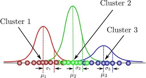
Gaussian mixture model is a soft clustering method. Each datapoint has a probability distribution of what cluster it may belong to.
 [2]
[2]
A Gaussian Mixture Model represents the probability density function of a dataset as:
$$ p(x) = \sum_{k=1}^{K} \pi_k\, \mathcal{N}(x \mid \mu_k, \Sigma_k) $$Non-negativity:
$$ \pi_k \geq 0 \quad \text{for all } k. $$
Normalization:
$$ \sum_{k=1}^{K} \pi_k = 1. $$
These properties ensure that each mixing coefficient represents a valid probability, indicating the prior probability that a randomly chosen data point comes from the corresponding Gaussian component.
The EM algorithm comprises two alternating steps:
In this step, the algorithm computes the "responsibilities" or the posterior probabilities that a data point $x^{(i)}$ belongs to each Gaussian component $k$. These responsibilities are denoted by $\gamma(z_{k}^{(i)})$ and are given by:
$$ \gamma(z_{k}^{(i)}) = \frac{\pi_k \, \mathcal{N}(x^{(i)} \mid \mu_k, \Sigma_k)}{\sum_{j=1}^{K} \pi_j \, \mathcal{N}(x^{(i)} \mid \mu_j, \Sigma_j)} $$In the M-Step, the parameters of the GMM (i.e., the mixing coefficients, means, and covariances) are updated to maximize the expected complete-data log-likelihood computed during the E-Step.
The update formulas are as follows:
Update the Mixing Coefficients:
$$ \pi_k = \frac{1}{N} \sum_{i=1}^{N} \gamma(z_{k}^{(i)}) $$
Here, $N$ is the total number of data points. This update computes the average responsibility for each component, effectively representing the proportion of the dataset assigned to component $k$.
Update the Means:
$$ \mu_k = \frac{\sum_{i=1}^{N} \gamma(z_{k}^{(i)}) \, x^{(i)}}{\sum_{i=1}^{N} \gamma(z_{k}^{(i)})} $$
This weighted average recalculates the center of the data assigned to each component.
Update the Covariance Matrices:
$$ \Sigma_k = \frac{\sum_{i=1}^{N} \gamma(z_{k}^{(i)}) \, (x^{(i)} - \mu_k)(x^{(i)} - \mu_k)^\top}{\sum_{i=1}^{N} \gamma(z_{k}^{(i)})} $$
The covariance update computes the weighted spread of the data around the updated mean for each component.
The EM algorithm proceeds as follows:
Initialization:
Choose initial values for the parameters $\{ \pi_k, \mu_k, \Sigma_k \}$, often by random assignment or using a clustering algorithm like K-means.
Iterative Updates:
Convergence:
The algorithm repeats these two steps until convergence. Convergence can be determined by:
import numpy as np
import matplotlib.pyplot as plt
from matplotlib.patches import Ellipse

# -------------------------------------------------------------------------
# 2. Plotting Function for Data and Gaussian Components
# -------------------------------------------------------------------------
def plot_gmm(X, means, covs, iteration, ax=None):
    """
    Plots the dataset along with the current Gaussian components.

    - Data points are plotted in grey.
    - The current means are marked with 'x' in different colors.
    - Each Gaussian's 1-standard-deviation ellipse is drawn.
    """
    if ax is None:
        fig, ax = plt.subplots(figsize=(8, 6))

    # Plot the dataset
    ax.scatter(X[:, 0], X[:, 1], s=10, alpha=0.5, color='grey')

    # Define colors for each component (you can customize these)
    colors = ['red', 'blue']
    for k, (mean, cov) in enumerate(zip(means, covs)):
        # Mark the mean
        ax.scatter(mean[0], mean[1], c=colors[k], s=100, marker='x')

        # Calculate eigenvalues and eigenvectors for the covariance matrix
        vals, vecs = np.linalg.eigh(cov)
        # Sort the eigenvalues in descending order for the correct ellipse shape
        order = vals.argsort()[::-1]
        vals = vals[order]
        vecs = vecs[:, order]
        angle = np.degrees(np.arctan2(vecs[1, 0], vecs[0, 0]))

        # The ellipse's width and height represent 2*sqrt(eigenvalue)
        width, height = 2 * np.sqrt(vals)
        ellip = Ellipse(xy=mean, width=width, height=height, angle=angle,
                        edgecolor=colors[k], facecolor='none', lw=2, label=f'Component {k+1}')
        ax.add_patch(ellip)

    ax.set_title(f'GMM - Iteration {iteration}')
    ax.legend()
    plt.show()

# -------------------------------------------------------------------------
# 3. Gaussian PDF and One EM Iteration
# -------------------------------------------------------------------------
def gaussian_pdf(x, mean, cov):
    """
    Computes the multivariate normal density for a given point x.
    """
    d = x.shape[0]
    norm_const = 1.0 / (np.power((2*np.pi), d/2) * np.sqrt(np.linalg.det(cov)))
    diff = (x - mean).reshape(-1, 1)
    exponent = -0.5 * (diff.T @ np.linalg.inv(cov) @ diff)[0, 0]
    return norm_const * np.exp(exponent)

def gmm_em_step(X, weights, means, covs):
    """
    Performs one iteration of the EM algorithm for the GMM.
    E-step: Compute responsibilities for each data point.
    M-step: Update weights, means, and covariances based on the responsibilities.

    Returns updated weights, means, covs, and the responsibilities matrix.
    """
    n_samples = X.shape[0]
    n_components = len(weights)
    # E-step: Compute responsibilities (soft assignments)
    responsibilities = np.zeros((n_samples, n_components))
    for i in range(n_samples):
        for k in range(n_components):
            responsibilities[i, k] = weights[k] * gaussian_pdf(X[i], means[k], covs[k])
        responsibilities[i, :] /= np.sum(responsibilities[i, :])

    # M-step: Update parameters using the responsibilities
    new_weights = np.zeros(n_components)
    new_means = []
    new_covs = []

    for k in range(n_components):
        Nk = np.sum(responsibilities[:, k])
        new_weights[k] = Nk / n_samples
        # Update mean: weighted average of data points
        new_mean = np.sum(responsibilities[:, k].reshape(-1, 1) * X, axis=0) / Nk
        new_means.append(new_mean)
        # Update covariance: weighted spread of the data around the new mean
        diff = X - new_mean
        new_cov = np.dot((responsibilities[:, k].reshape(-1, 1) * diff).T, diff) / Nk
        new_covs.append(new_cov)

    return new_weights, np.array(new_means), new_covs, responsibilities

# -------------------------------------------------------------------------
# 4. Running the GMM Demo
# -------------------------------------------------------------------------
def run_gmm_demo(n_iterations=10):
    """
    Generates the dataset, initializes the GMM parameters, and then
    iteratively runs the EM algorithm while plotting the progress.
    """
    # Generate the dataset
    X = generate_data()
    n_components = 2  # We know we have 2 clusters

    # Initialize GMM parameters
    weights = np.array([0.5, 0.5])
    # For means, randomly select two data points from the dataset
    np.random.seed(0)
    indices = np.random.choice(X.shape[0], n_components, replace=False)
    means = X[indices]
    # Initialize covariances with the overall covariance of the dataset
    overall_cov = np.cov(X, rowvar=False)
    covs = [overall_cov for _ in range(n_components)]

    # Iterate the EM algorithm and plot the outcome at each iteration
    for iteration in range(n_iterations):
        weights, means, covs, responsibilities = gmm_em_step(X, weights, means, covs)
        plot_gmm(X, means, covs, iteration + 1)

# Run the demonstration
run_gmm_demo(n_iterations=10)


[1] Kamper, Herman "K-means clustering [lectures]" - https://youtu.be/_Tf1Vi4s7Ec&list=PLmZlBIcArwhMfNuMBg4XR-YQ0QIqdHCrl
[2] Carrasco, Oscar "Gaussian Mixture Model Explained" - https://builtin.com/articles/gaussian-mixture-model