Things we'll cover in today's lecture:
- Revisit computation graphs
- Assorted matrix operations
Motivation
Motivation:
What are we hoping to learn?
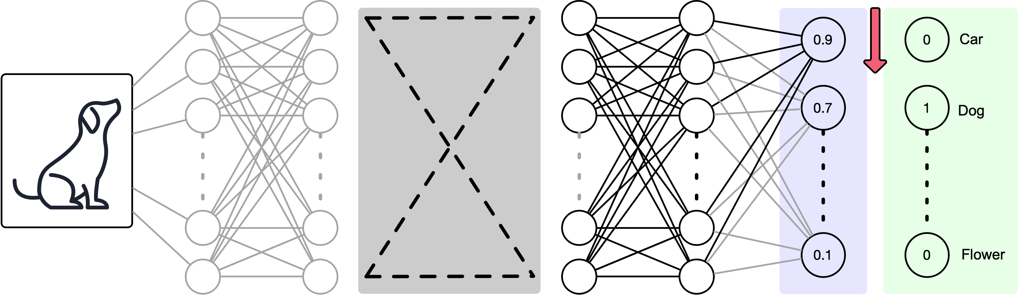
Let's think of a convolutional neural network we see in literature. We input a image and get out the probability that the image is one of several classifications:
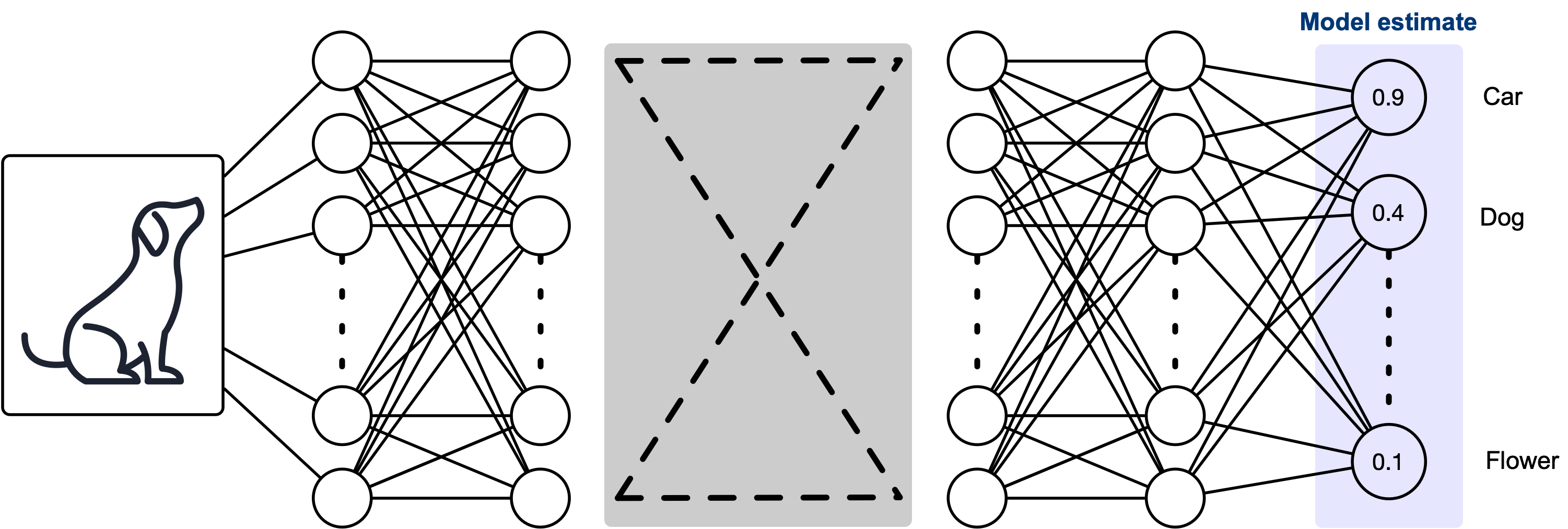
Ofcourse, there is a ground truth that we need to consider. Model seems off?
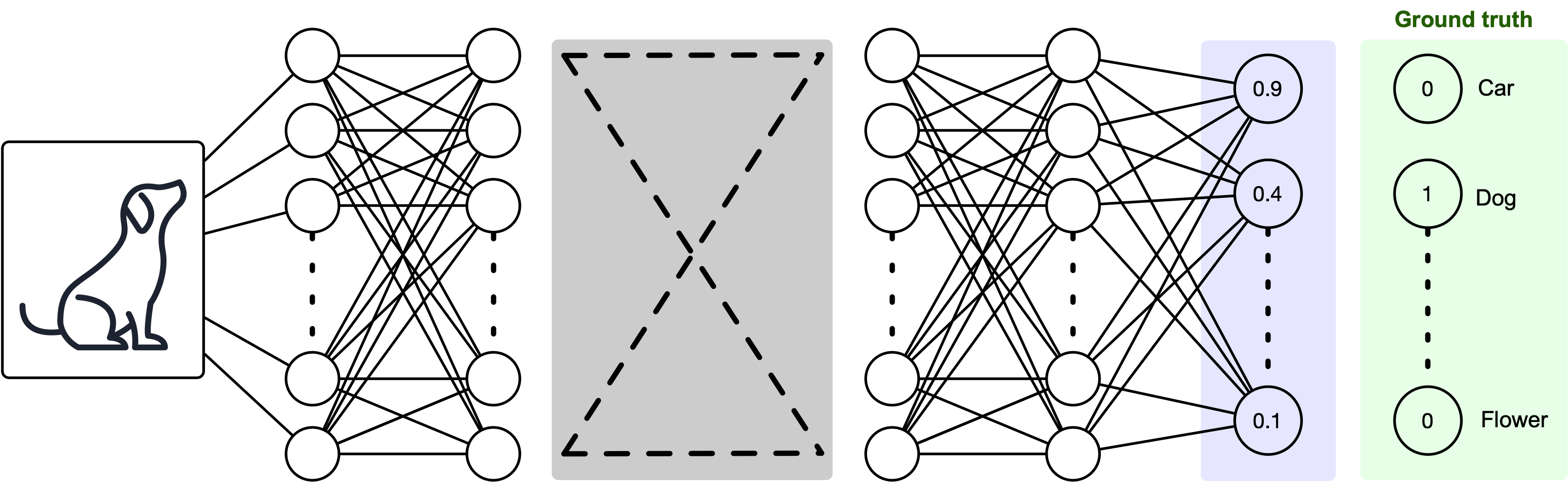
The output layer needs to be corrected according to the model errors.
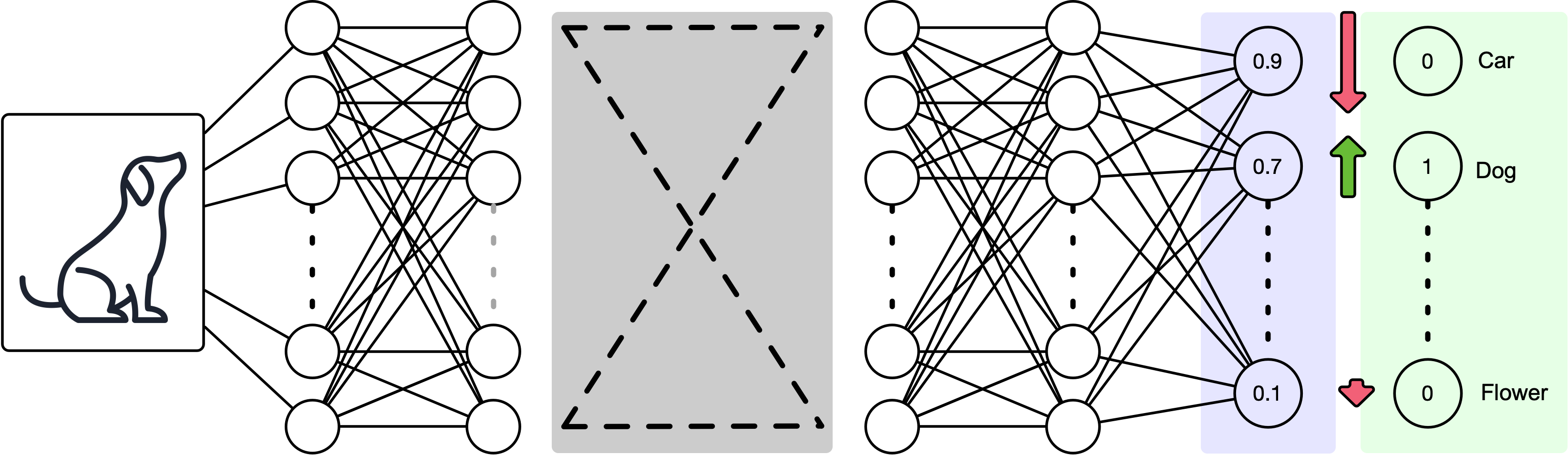
Which means the prior layer should also be adjusted according to the error in the output layer.
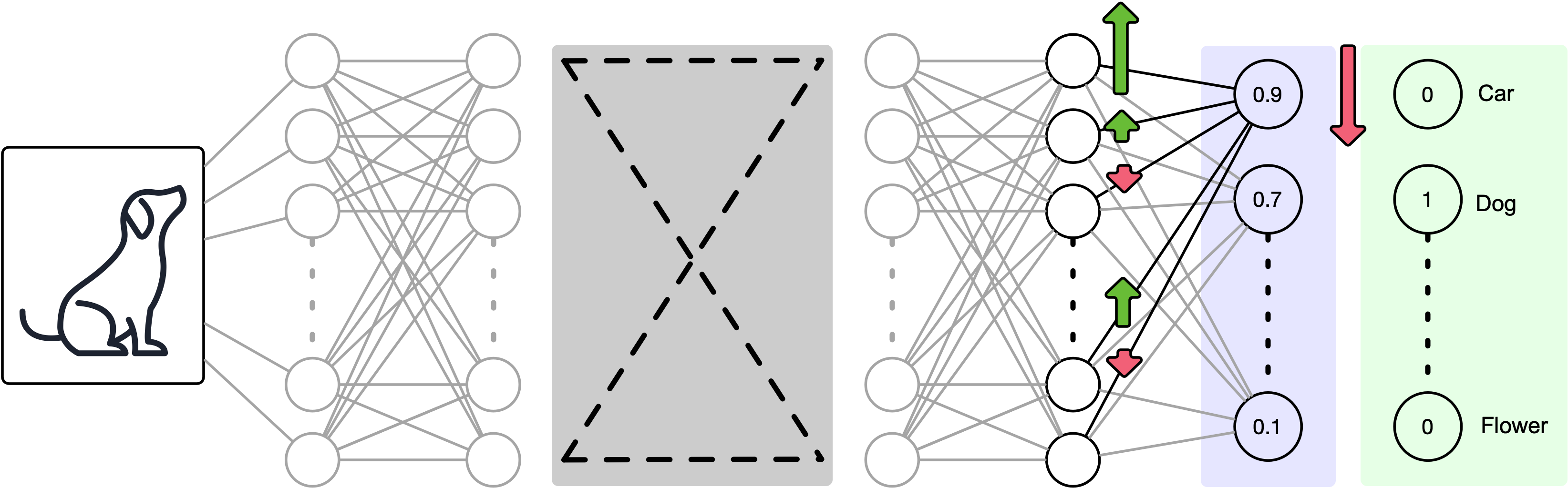
And we adjust back accordingly.
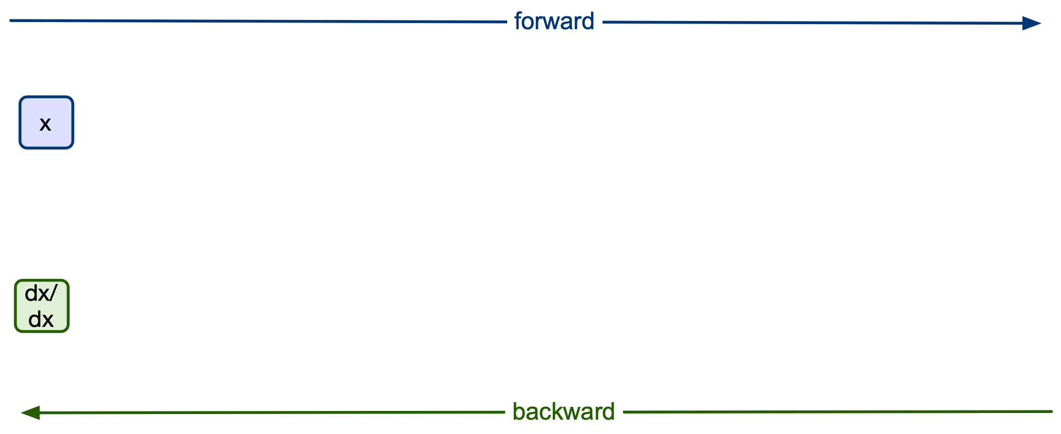
How computation graphs work (in PyTorch)
Let's reconsider the simple network we talked about in last lecture.
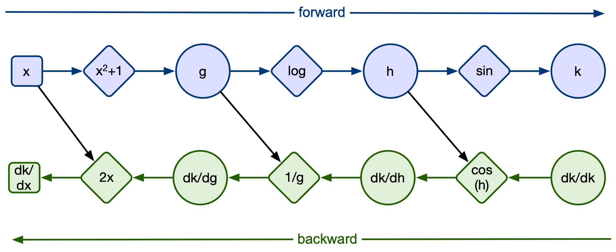
Remember we had a multi-function network:

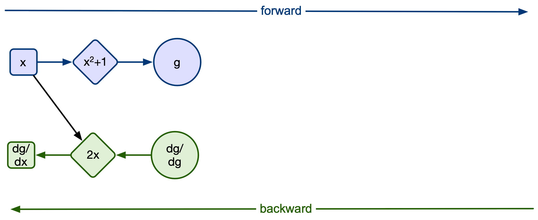
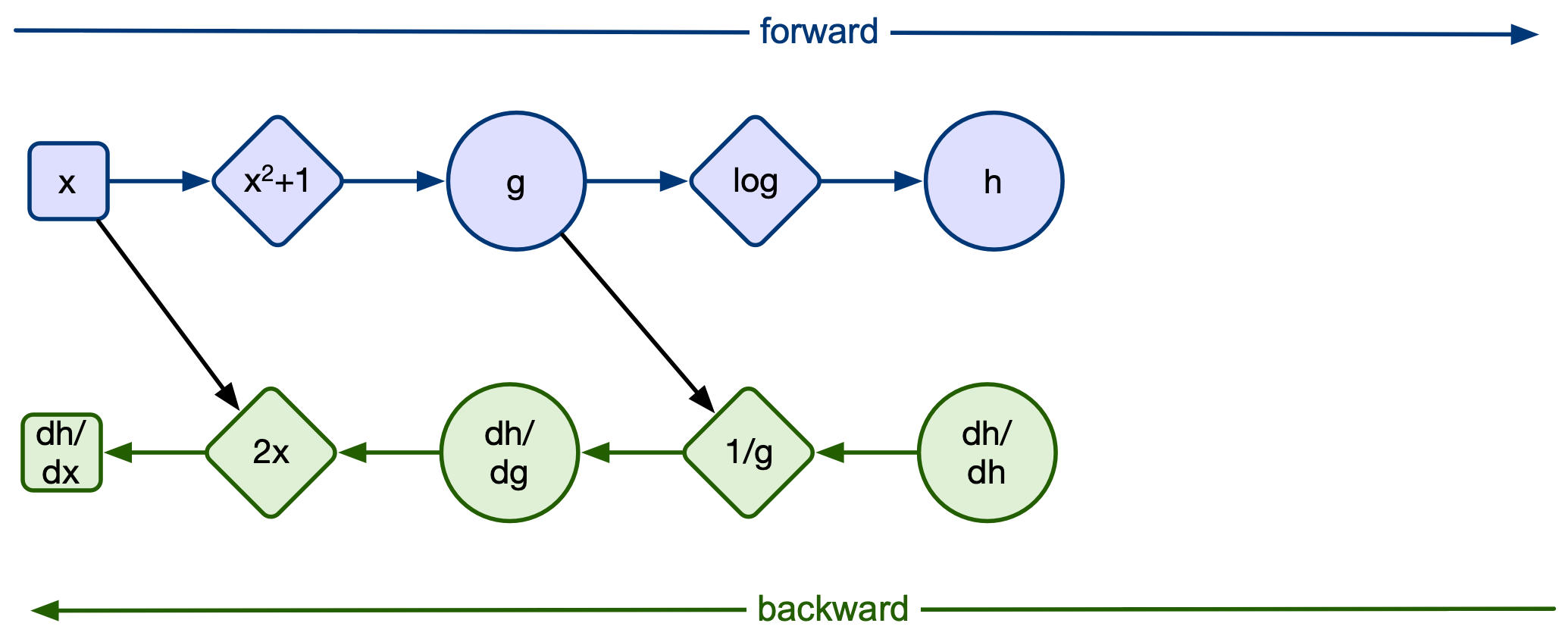
Where the functions above are defined as follows:
$g(x) = x^2+1$, $h(g) = \log(g)$, $k(h) = \sin(h)$. Thus, $f(x) = k(h(g(x)))$
The resulting function is: $$f(x) = \sin(\log(((x)^2+1)))$$
import torch

# Function to compute y = sin(log(x^2 + 1))
def func(x):
    g = x**2 + 1
    h = torch.log(g)
    k = torch.sin(h)
    return k
    #return torch.sin(torch.log(x**2 + 1))

# Set up the initial guess for x (starting point for optimization)
x = torch.tensor([1.0], requires_grad=True)  # x is a scalar, requires gradients

# Use an optimizer to minimize the difference between y and 0
optimizer = torch.optim.Adam([x], lr=0.1)

# Number of iterations for optimization
num_iterations = 10

for i in range(num_iterations):
    # Zero the gradients from the previous step
    optimizer.zero_grad()

    # Compute the function value
    y = func(x)

    print(x)
    # Compute the loss, we want to find x when y = 0
    loss = y**2  # This is the squared error between y and 0

    #Calculate manual gradient of x
    manual = 2*x*torch.cos(torch.log(x**2+1))/(x**2+1)

    # Perform backward propagation to compute the gradients
    y.backward()

    # Print the current value of x and loss at every 100 iterations
    if i % 1 == 0:
        print(f"Iteration {i}, x: {x.item():.4f}, y: {y.item():.6f}, Auto Gradient of x: {x.grad.item():.6f}, Manual Gradient of x: {manual.item():.6f}")

    # Update the value of x using the optimizer
    optimizer.step()

# Final value of x where y should be approximately 0
print(f"Final value of x: {x.item():.4f}")
tensor([1.], requires_grad=True)
Iteration 0, x: 1.0000, y: 0.638961, Auto Gradient of x: 0.769239, Manual Gradient of x: 0.769239
tensor([0.9000], requires_grad=True)
Iteration 1, x: 0.9000, y: 0.559122, Auto Gradient of x: 0.824505, Manual Gradient of x: 0.824505
tensor([0.7999], requires_grad=True)
Iteration 2, x: 0.7999, y: 0.474661, Auto Gradient of x: 0.858673, Manual Gradient of x: 0.858673
tensor([0.6996], requires_grad=True)
Iteration 3, x: 0.6996, y: 0.387947, Auto Gradient of x: 0.865841, Manual Gradient of x: 0.865841
tensor([0.5992], requires_grad=True)
Iteration 4, x: 0.5992, y: 0.301997, Auto Gradient of x: 0.840632, Manual Gradient of x: 0.840632
tensor([0.4989], requires_grad=True)
Iteration 5, x: 0.4989, y: 0.220408, Auto Gradient of x: 0.779257, Manual Gradient of x: 0.779257
tensor([0.3989], requires_grad=True)
Iteration 6, x: 0.3989, y: 0.147134, Auto Gradient of x: 0.680803, Manual Gradient of x: 0.680803
tensor([0.3000], requires_grad=True)
Iteration 7, x: 0.3000, y: 0.086076, Auto Gradient of x: 0.548428, Manual Gradient of x: 0.548428
tensor([0.2032], requires_grad=True)
Iteration 8, x: 0.2032, y: 0.040449, Auto Gradient of x: 0.389961, Manual Gradient of x: 0.389961
tensor([0.1100], requires_grad=True)
Iteration 9, x: 0.1100, y: 0.012033, Auto Gradient of x: 0.217409, Manual Gradient of x: 0.217409
Final value of x: 0.0226
So the major question is how does the computer keep track of the gradient calculation?
Through computation graphs! But how does PyTorch create computation graphs? Let's go through the prior example:
Good references:
Starting off with x we need to tell PyTorch to create a new computation graph. We do this by turning on the requires_grad option of the tensor:
x = torch.tensor([1.0], requires_grad=True)
x
tensor([1.], requires_grad=True)
Under the hood, whats happening is that the requires_grad option allocates a AutogradMeta object that stores the graph information. The graph stores derivative functions and values.
Next we define the next step in our composite function g(x). The resulting tensor has a pointer to a field called grad_fn which is function that will be used to calculate the backward gradient.
g1 = x**2
print(g1)
g = g1+1
print(g)
tensor([1.], grad_fn=<PowBackward0>)
tensor([2.], grad_fn=<AddBackward0>)
Notice that even though g(x) is defined in one line, it contains two backward functions. A backward function is inserted into the graph whenever a new operation is performed on a tensor with a gradient activation flag.
PyTorch has a file called tools/autograd/derivatives/yaml that stores the derivatives of many (most?) functions you will see (you can manually define a custom function/derivative yourself as well!)
Next we want to define the log function:
h = torch.log(g)
print(h)
tensor([0.6931], grad_fn=<LogBackward0>)
Finally we define the sin function:
k = torch.sin(h)
print(k)
tensor([0.6390], grad_fn=<SinBackward0>)
As mentioned earlier we can view the network using the tensorboard utility
import torch
from torch.utils.tensorboard import SummaryWriter
writer = SummaryWriter('runs/experiment_2')
class OurNet(torch.nn.Module):
    def __init__(self):
        super(OurNet,self).__init__()
    def forward(self,x):
        g1 = x**2
        g = g1 + 1
        h = torch.log(g)
        k = torch.sin(h)
        return k
graph = OurNet()
writer.add_graph(graph,torch.randn((1)))
writer.close()

### use tensorboard --logdir=runs command to view
Live tensorboard demo
So now that we understand computation graphs, how do we get from:
to:
Linear Algebra for Machine Learning
Linear algebra is a core mathematical concept in machine learning, especially deep learning
Scaler, vector, matrix and tensor (Review)
- Scaler - A scalar is a single number
- Vector - 1-D list of numbers
- Matrix - 2-D list of numbers
- Tensor - N-D list of numbers

- We refer to anything which has three or more dimensions as a tensor rather than a matrix.
Matrix Transpose
The transpose of a matrix is found by switching its rows with its columns. The transpose of the matrix can be thought of as a mirror image across the main diagonal.
$A=\left[\begin{matrix}a_{11} & a_{12} & \ldots & a_{1n}\
a_{21} & a_{22} & \vdots & a_{2n}\
\vdots & \vdots & \ddots & \vdots\
a_{m1} & a_{m2} & \ldots & a_{mn}
\end{matrix}\right]$;<Br>
__Transpose matrix:__ $A^{T}=\left[\begin{matrix}a_{11} & a_{21} & \ldots & a_{m1}\\
a_{12} & a_{22} & \vdots & a_{m2}\\
\vdots & \vdots & \ddots & \vdots\\
a_{1n} & a_{2n} & \ldots & a_{mn}
\end{matrix}\right]$
- In Pytorch you can transpose a matrix in two ways: torch.t() or torch.transpose()
import torch
a = torch.tensor([
    [1, 2, 3],
    [1, 2, 3]
])
transpose_a = torch.t(a)
print("Transpose matrix of a is",transpose_a)
Transpose matrix of a is tensor([[1, 1],
        [2, 2],
        [3, 3]])
transpose_a = torch.transpose(a,0,1)
print("Transpose matrix of a is",transpose_a)
Transpose matrix of a is tensor([[1, 1],
        [2, 2],
        [3, 3]])
Inner (dot) product of two vectors
- The inner product takes two vectors of equal size and returns a single number (scalar). This is calculated by multiplying the corresponding elements in each vector and adding up all of those products.
- For example: $\left[\begin{array}{c}
1\ 2\ 3 \end{array}\right]\cdot\left[\begin{array}{c} 4\\ 5\\ 6 \end{array}\right]=1\times4+2\times5+3\times6=32$
- In Pytorch we use torch.dot() to calculate innder product of the vectors that are the same size.
import torch
a = torch.tensor([1, 2, 3])
b = torch.tensor([4, 5, 6])

ab= torch.dot(a, b)
print (a)
print (b)
print ("Inner product of a and b is",ab)
tensor([1, 2, 3])
tensor([4, 5, 6])
Inner product of a and b is tensor(32)
- This operation is also commutative, in which $\boldsymbol{a}\cdot\boldsymbol{b}=\boldsymbol{b}\cdot\boldsymbol{a}$
ba= torch.dot(b, a)
print ("Inner product of b and a is",ba)
Inner product of b and a is tensor(32)
# what if now the vectors are not the same size
a = torch.tensor([1, 2])
c = torch.tensor([3, 2, 1])

ac= torch.dot(a, c)
print ("Inner product of a and b is",ac)
Matrix-Vector dot product
Multiplication between a matrix $A$ and vector $x$ is given as:
$Ax = \left[ \begin{matrix} a_{11} & a_{12} & \ldots & a_{1n} \\ a_{21} & a_{22} & \vdots & a_{2n} \\ \vdots & \vdots & \ddots & \vdots \\ a_{m1} & a_{m2} & \ldots & a_{mn} \end{matrix} \right] \left[ \begin{matrix} x_{1} \\ x_{2} \\ \vdots \\ x_{n} \end{matrix} \right] = \left[ \begin{matrix} a_{11} x_{1} + a_{12} x_{2} + \ldots + a_{1n} x_{n} \\ a_{21} x_{1} + a_{22} x_{2} + \ldots + a_{2n} x_{n} \\ \ldots \\ a_{m1} x_{1} + a_{m2} x_{2} + \ldots + a_{mn} x_{n} \end{matrix} \right]$
This method computes matrix dot product with a vector by taking an 𝑚×𝑛 2D Tensor (matrix) and an 𝑛 1D Tensor (vector). The result is a m 1D Tensor (vector).
In Pytorch we use torch.Mv() to calculate dot product of the a 2D matrix and a vector.
import torch
a  =  torch.randn(2, 3)
b  =  torch.randn(3)
print(a)
print(b)
c = torch.mv(a,b)
print("Matrix-vector dot product is",c)
tensor([[-1.0917,  0.6832,  1.5545],
        [-1.0927,  0.6571,  0.5402]])
tensor([-0.2527, -0.5882, -2.8065])
Matrix-vector dot product is tensor([-4.4887, -1.6265])
d = a@b
print("Matrix multiplication is", d)
Matrix multiplication is tensor([-4.4887, -1.6265])
Wait a minute, if torch.mm and torch.mv do the same thing, why does torch.mv even exist? `
Speed
import torch
import time

# Define the size of the matrix and vector
m, n = 1000, 1000

# Create a random matrix A (m x n) and a random vector v (n,)
A = torch.rand(m, n)
v = torch.rand(n)

# Time `torch.mv` (matrix-vector multiplication)
start_time = time.time()
result_mv = torch.mv(A, v)
mv_time = time.time() - start_time

# Time `torch.mm` (matrix-matrix multiplication)
start_time = time.time()
# We need to reshape v to be a matrix with shape (n, 1) for mm
result_mm = torch.mm(A, v.view(-1, 1))
mm_time = time.time() - start_time

# Print the results
print(f"Time taken by torch.mv: {mv_time:.6f} seconds")
print(f"Time taken by torch.mm: {mm_time:.6f} seconds")
Time taken by torch.mv: 0.009708 seconds
Time taken by torch.mm: 0.012335 seconds
Hadamard Product (Element Wise Multiplication)
- Hadamard product of two vectors/matrices is very similar to matrix addition, elements corresponding to same row and columns of given vectors/matrices are multiplied together to form a new vector/matrix.
- The order of matrices/vectors to be multiplied should be same and the resulting matrix will also be of same order.
- Example: $\left[\begin{array}{cc}
1 & 2\ 3 & 4 \end{array}\right]\circ\left[\begin{array}{cc} 5 & 6\\ 7 & 8 \end{array}\right]=\left[\begin{array}{cc} \left(1\times5\right) & \left(2\times6\right)\\ \left(3\times7\right) & \left(4\times8\right) \end{array}\right]=\left[\begin{array}{cc} 5 & 12\\ 21 & 32 \end{array}\right]$
import torch
a = torch.tensor([[1, 2],[3, 4]])
b = torch.tensor([[5, 6],[7, 8]])

ab = a*b
print (a)
print (b)
print ("Hadamard product of a and b is",ab)
tensor([[1, 2],
        [3, 4]])
tensor([[5, 6],
        [7, 8]])
Hadamard product of a and b is tensor([[ 5, 12],
        [21, 32]])
Matrix dot product
- Dot product of two matrices requires the matrices to have certain sizes. The number of columns of the first matrix must be equal to the number of rows of the second matrix. Each row of the first matrix will be transposed and multiplied against each column in the second matrix. This is basically a vector multiplication where each row in the first matrix is transposed to make sure it has the same dimension as each column in the second matrix.
- For example:
$\left[\begin{array}{cc} 1 & 2\\ 3 & 4\\ 5 & 6 \end{array}\right]\cdot\left[\begin{array}{ccc} {\color{brown}1} & {\color{brown}2} & {\color{brown}3}\\ {\color{brown}4} & {\color{brown}5} & {\color{brown}6} \end{array}\right]=\left[\begin{array}{ccc} \left(1\times{\color{brown}1}+2\times{\color{brown}4}\right) & \left(1\times{\color{brown}2}+2\times{\color{brown}5}\right) & \left(1\times{\color{brown}3}+2\times{\color{brown}6}\right)\\ \left(3\times{\color{brown}1}+4\times{\color{brown}4}\right) & \left(3\times{\color{brown}2}+4\times{\color{brown}5}\right) & \left(3\times{\color{brown}3}+4\times{\color{brown}6}\right)\\ \left(5\times{\color{brown}1}+6\times{\color{brown}4}\right) & \left(5\times{\color{brown}2}+6\times{\color{brown}5}\right) & \left(5\times{\color{brown}3}+6\times{\color{brown}6}\right) \end{array}\right]=\left[\begin{array}{ccc} 9 & 12 & 15\\ 19 & 26 & 33\\ 29 & 40 & 51 \end{array}\right]$
- In Pytorch we use torch.mm() to calculate Dot product of two 2-dimentional matrices. This method computes matrix dot product by taking an 𝑚×𝑛 Tensor and an 𝑛×𝑝 Tensor. It can deal with only two-dimensional matrices and not with single-dimensional ones. This function does not support broadcasting. Broadcasting is nothing but the way the tensors are treated when their shapes are different. The smaller Tensor is broadcasted to suit the shape of the wider or larger Tensor for operations.
# Example of matrix dot product
a = torch.arange(1, 7).view(2, 3)
b = torch.arange(1, 7).view(3, 2)
print(a)
print(b)
adotb=torch.mm(a, b)
print ("Dot product of a and b is",adotb)
tensor([[1, 2, 3],
        [4, 5, 6]])
tensor([[1, 2],
        [3, 4],
        [5, 6]])
Dot product of a and b is tensor([[22, 28],
        [49, 64]])
# Example of matrix dot product
a = torch.arange(1, 7).view(3, 2)
b = torch.arange(1, 7).view(2, 3)
print(a)
print(b)
adotb=torch.mm(a, b)
print ("Dot product of a and b is")
print (adotb)
tensor([[1, 2],
        [3, 4],
        [5, 6]])
tensor([[1, 2, 3],
        [4, 5, 6]])
Dot product of a and b is
tensor([[ 9, 12, 15],
        [19, 26, 33],
        [29, 40, 51]])
- Unlike inner product, matrix multiplication is not commutative, in which $\boldsymbol{a}\cdot\boldsymbol{b}\neq\boldsymbol{b}\cdot\boldsymbol{a}$
# Matrix multiplication is not commutative,
bdota=torch.mm(b, a)
print ("Dot product of b and a is",bdota)
- Example below shows that it is important to make sure the rows of the first matrix have the same number of entries as the columns of the second matrix.
# the dimensions of the matrices is important for matrix multiplication
adota=torch.mm(a, a)
print ("Dot product of a and a is",adota)
---------------------------------------------------------------------------
RuntimeError                              Traceback (most recent call last)
Cell In[34], line 2
      1 # the dimensions of the matrices is important for matrix multiplication
----> 2 adota=torch.mm(a, a)
      3 print ("Dot product of a and a is",adota)

RuntimeError: mat1 and mat2 shapes cannot be multiplied (3x2 and 3x2)
Matrix product of two tensors (general form)
- In Pytorch we use torch.matmul(Tensor_1, Tensor_2, out=None) to compute the multiplication of two vector matrices (single-dimensional matrices), 2D matrices and mixed ones also. This method also supports broadcasting and batch operations. Depending upon the input matrices dimensions, the operation to be done is decided.
- The table below lists the various possible dimensions of the arguments and the operations based on it.
| Argument 1 | Argument 2 | Action taken |
|---|---|---|
| 1-dimensional | 1-dimensional | The scalar product is calculated |
| 2-dimensional | 2-dimensional | General matrix multiplication is done |
| 1-dimensional | 2-dimensional | The tensor 1 is pretended with a ‘1’ to match dimension of tensor 2 |
| 2-dimensional | 1-dimensional | Matrix-vector product is calculated |
| 1/N-dimensional (N>2) | 1/N-dimensional (N>2) | Batched matrix multiplication is done |
# both arguments 1D
vec_1 = torch.tensor([3, 6, 2])
vec_2 = torch.tensor([4, 1, 9])

print("Single dimensional tensors :", torch.matmul(vec_1, vec_2))
Single dimensional tensors : tensor(36)
# both arguments 2D
mat_1 = torch.tensor([[1, 2, 3],
                      [4, 3, 8],
                      [1, 7, 2]])

mat_2 = torch.tensor([[2, 4, 1],
                      [1, 3, 6],
                      [2, 6, 5]])

out = torch.matmul(mat_1, mat_2)

print("\n3x3 dimensional tensors :\n", out)
3x3 dimensional tensors :
 tensor([[10, 28, 28],
        [27, 73, 62],
        [13, 37, 53]])
# Arguments of different dimensions
# first argument 1D and second argument 2D
mat1_1 = torch.tensor([3, 6, 2])

mat1_2 = torch.tensor([[1, 2, 3],
                       [4, 3, 8],
                       [1, 7, 2]])

out_1 = torch.matmul(mat1_1, mat1_2)
print("\n1D-2D multiplication :\n", out_1)
1D-2D multiplication :
 tensor([29, 38, 61])
# first argument 2D and second argument 1D
mat2_1 = torch.tensor([[2, 4, 1],
                       [1, 3, 6],
                       [2, 6, 5]])

mat2_2 = torch.tensor([4, 1, 9])

# assigning to output tensor
out_2 = torch.matmul(mat2_1, mat2_2)

print("\n2D-1D multiplication :\n", out_2)
2D-1D multiplication :
 tensor([21, 61, 59])
# N-dimensional argument (N>2)
# creating Tensors using randn()
mat_1 = torch.randn(2, 3, 3)
mat_2 = torch.randn(3)

# printing the matrices
print("matrix A :\n", mat_1)
print("\nmatrix B :\n", mat_2)

# output
print("\nOutput :\n", torch.matmul(mat_1, mat_2))
matrix A :
 tensor([[[ 1.9742, -0.3101,  0.9207],
         [-0.5845,  0.3964,  0.2774],
         [ 0.1423, -0.6356, -1.0601]],

        [[ 0.7488,  0.0633, -0.1190],
         [ 0.2655, -1.8284, -1.4647],
         [ 0.2355, -0.5253,  0.6223]]])

matrix B :
 tensor([ 0.7186, -1.4878,  1.3330])

Output :
 tensor([[ 3.1072, -0.6399, -0.3651],
        [ 0.2852,  0.9588,  1.7803]])
That's it for today
Next time we will discuss more advanced linear algebra topics before moving onto auto-differentiation!