Lecture 21 - Words and Attention (aka the basic transformer model)

ECE364 - Programming Methods for Machine Learning

Nickvash Kani

Slides based off prior lectures by Alex Schwing, Aigou Han, Farzad Kamalabadi, Corey Snyder. All mistakes are my own!

In this lecture:

• Discuss the basic structure of the trasnformer model
• Discuss embeddings

Where did we leave language processing?

When we last talked about generating language, it was with recurrent neural networks:

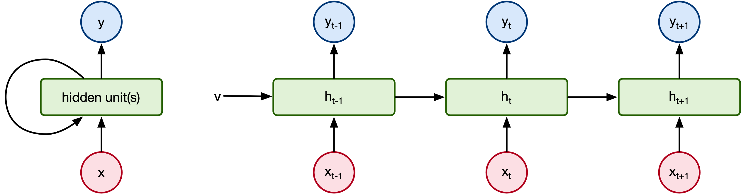
But there are problems with simple RNNs:

• Slow - RNNs process data sequentially making them super slow.
• Vanishing gradient - RNNs (including LSTMs and GRUs) struggle with learning long range dependencies due to vanishing gradients. [1]
• Lack of attention - RNNs process each word in order, and have difficulty with non-sequential dependencies.

Attention is all you need

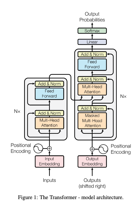
In 2017, Ashish Vaswani and his colleagues at Google Research/Brain published their seminal work "Attention is all you need" [2]. In it, they introduce the transformer architecture which has become the foundation of every large language model since. So in this lecture, let's go through and try to decipher this architecture:

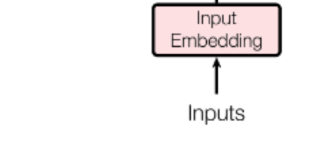
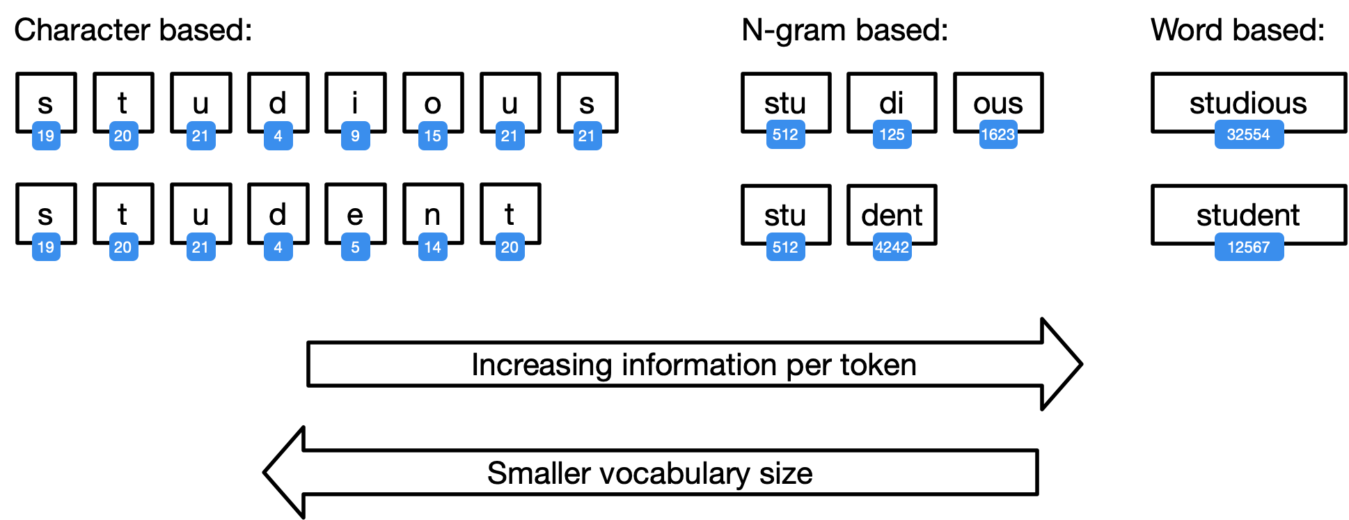
Step 1: Tokenization

We brushed on tokenization previously, but the basic idea is that you can segment language by letters, words, or something in between. What features you use can significantly impact your model's performance and structure.

import torch
from transformers import AutoTokenizer, AutoModelForCausalLM

# Load a tiny GPT-2 model (small enough for CPU)
tokenizer = AutoTokenizer.from_pretrained("distilgpt2")
model = AutoModelForCausalLM.from_pretrained("distilgpt2")

# Make sure model is in eval mode
model.eval()

/Users/nvk/opt/anaconda3/envs/ece364_oldnb/lib/python3.11/site-packages/tqdm/auto.py:21: TqdmWarning: IProgress not found. Please update jupyter and ipywidgets. See https://ipywidgets.readthedocs.io/en/stable/user_install.html
  from .autonotebook import tqdm as notebook_tqdm

GPT2LMHeadModel(
  (transformer): GPT2Model(
    (wte): Embedding(50257, 768)
    (wpe): Embedding(1024, 768)
    (drop): Dropout(p=0.1, inplace=False)
    (h): ModuleList(
      (0-5): 6 x GPT2Block(
        (ln_1): LayerNorm((768,), eps=1e-05, elementwise_affine=True)
        (attn): GPT2Attention(
          (c_attn): Conv1D(nf=2304, nx=768)
          (c_proj): Conv1D(nf=768, nx=768)
          (attn_dropout): Dropout(p=0.1, inplace=False)
          (resid_dropout): Dropout(p=0.1, inplace=False)
        )
        (ln_2): LayerNorm((768,), eps=1e-05, elementwise_affine=True)
        (mlp): GPT2MLP(
          (c_fc): Conv1D(nf=3072, nx=768)
          (c_proj): Conv1D(nf=768, nx=3072)
          (act): NewGELUActivation()
          (dropout): Dropout(p=0.1, inplace=False)
        )
      )
    )
    (ln_f): LayerNorm((768,), eps=1e-05, elementwise_affine=True)
  )
  (lm_head): Linear(in_features=768, out_features=50257, bias=False)
)

from transformers import AutoTokenizer

tokenizer = AutoTokenizer.from_pretrained("distilgpt2")

text = "The quick brown fox"
input_ids = tokenizer.encode(text)
tokens = tokenizer.tokenize(text)
words = [tokenizer.decode([id]) for id in input_ids]

print("Token IDs: ")
print(input_ids)
print("Tokens: ")
print(tokens)
print("Decoded tokens: ")
print(words)
print(f"Number of tokens: {len(tokens)}")

Token IDs: 
[464, 2068, 7586, 21831]
Tokens: 
['The', 'Ġquick', 'Ġbrown', 'Ġfox']
Decoded tokens: 
['The', ' quick', ' brown', ' fox']
Number of tokens: 4

Concept	Explanation
Token $\neq$ Word	A word may be split into multiple tokens if it’s rare/complex.
Special Space Tokens	GPT-2 uses a Ġ (special marker) to represent leading spaces in tokens.
Number of tokens	Depends on how text is broken into subwords.
In this case	"The quick brown fox" tokenizes to

Inference

How would we generate a totally new sequence from the transformer?

First let's look at what we get when we insert a input sequence into the model:

input_ids = tokenizer.encode("The quick brown fox", return_tensors='pt').to('cpu')
print(input_ids)

# Forward pass through model
with torch.no_grad():
    outputs = model(input_ids)
    logits = outputs.logits  # (batch_size, seq_length, vocab_size)
    
print(logits.shape)
print(logits)

tensor([[  464,  2068,  7586, 21831]])
torch.Size([1, 4, 50257])
tensor([[[-31.6921, -29.4775, -31.2145,  ..., -42.1520, -42.1397, -31.2937],
         [-45.3960, -46.4871, -50.1948,  ..., -53.8671, -52.9930, -48.0212],
         [-47.8363, -49.3172, -53.7016,  ..., -58.7728, -55.6532, -52.6001],
         [-56.9420, -58.9452, -61.8929,  ..., -68.8899, -63.3963, -60.5468]]])

What do the logits represent?

You can think of the logit matrix will be of the form: [batch_size, sequence_length, vocab_size]

Each slice logits[:, i, :] (for some $i$) represents the model’s prediction of what token should come next after the $i$-th token.

Specifically:

• logits[:, 0, :] → predict what comes after the first token
• logits[:, 1, :] → predict what comes after the second token
• logits[:, 2, :] → predict what comes after the third token
• ...
• logits[:, -1, :] → predict what comes after the very last token you input

That's why when generating the next token, you only care about the last position — logits[:, -1, :].

It’s predicting the next token based on the full context so far.

How do we generate a long sequence?

So let's generate a long sequence.

def generate_step(model, tokenizer, input_text, device='cpu'):
    """
    Given the current input_text, run one generation step.
    - Return updated text
    - Return top 10 next-token candidates (token, probability)
    """
    # Tokenize input
    input_ids = tokenizer.encode(input_text, return_tensors='pt').to(device)

    # Forward pass through model
    with torch.no_grad():
        outputs = model(input_ids)
        logits = outputs.logits  # (batch_size, seq_length, vocab_size)

    # Focus on the last token's logits
    next_token_logits = logits[:, -1, :].squeeze(0)  # (vocab_size,)

    # Convert logits to probabilities
    probs = torch.softmax(next_token_logits, dim=-1)

    # Get top 10 most probable tokens
    top_probs, top_indices = torch.topk(probs, 10)

    # Decode top tokens
    top_tokens = [tokenizer.decode(idx.item()) for idx in top_indices]

    # Greedy choice: pick the token with the highest probability
    next_token_id = top_indices[0].unsqueeze(0)
    next_token = tokenizer.decode(next_token_id)

    # Append the new token to the existing text
    updated_text = input_text + next_token

    # Prepare top 10 as a list of (token, probability) pairs
    top_10 = [(token, prob.item()) for token, prob in zip(top_tokens, top_probs)]

    return updated_text, top_10

# Initial prompt
text = "The meaning of life is"

# Generation steps
for _ in range(5):
    text, top_10 = generate_step(model, tokenizer, text)
    print("Top 10 next tokens:")
    for token, prob in top_10:
        print(f"{token!r} ({prob:.4f})")
    print(f"Updated Text: {repr(text)}\n")
    print("\n" + "-"*50 + "\n")

Top 10 next tokens:
' to' (0.1513)
' not' (0.0890)
' a' (0.0650)
' that' (0.0557)
' the' (0.0513)
' defined' (0.0199)
' an' (0.0157)
',' (0.0153)
' one' (0.0118)
' in' (0.0112)
Updated Text: 'The meaning of life is to'


--------------------------------------------------

Top 10 next tokens:
' be' (0.2613)
' live' (0.0408)
' say' (0.0191)
' have' (0.0159)
' make' (0.0149)
' give' (0.0130)
' know' (0.0123)
' find' (0.0119)
' the' (0.0110)
' take' (0.0099)
Updated Text: 'The meaning of life is to be'


--------------------------------------------------

Top 10 next tokens:
' understood' (0.0404)
' able' (0.0314)
' a' (0.0283)
' lived' (0.0276)
' the' (0.0231)
' found' (0.0166)
' determined' (0.0162)
' seen' (0.0150)
' defined' (0.0135)
' in' (0.0130)
Updated Text: 'The meaning of life is to be understood'


--------------------------------------------------

Top 10 next tokens:
' as' (0.2249)
' in' (0.1128)
' and' (0.0959)
' by' (0.0883)
',' (0.0871)
'.' (0.0610)
' to' (0.0374)
' through' (0.0241)
' only' (0.0229)
' not' (0.0198)
Updated Text: 'The meaning of life is to be understood as'


--------------------------------------------------

Top 10 next tokens:
' a' (0.2281)
' the' (0.1354)
' being' (0.1226)
' an' (0.0528)
' having' (0.0266)
' one' (0.0259)
' something' (0.0250)
' life' (0.0233)
',' (0.0157)
' living' (0.0121)
Updated Text: 'The meaning of life is to be understood as a'


--------------------------------------------------

Any guesses what the meaning of life is to DistilGPT2?

def generate_n_tokens(model, tokenizer, input_text, n_tokens=5, device='cpu', verbose=True):
    """
    Generate `n_tokens` tokens from input_text using greedy decoding.
    - verbose=True prints generation steps
    - returns the final updated text
    """
    text = input_text

    for i in range(n_tokens):
        text, top_10 = generate_step(model, tokenizer, text, device=device)

        if verbose:
            print(f"Step {i+1}:")
            print(f"Updated Text: {repr(text)}\n")
            print("Top 10 next tokens:")
            for token, prob in top_10:
                print(f"{token!r} ({prob:.4f})")
            print("\n" + "-"*50 + "\n")

    return text

start_text = "The meaning of life is to"
final_text = generate_n_tokens(model, tokenizer, start_text, n_tokens=20, verbose=False)
print("Final generated text:\n", final_text)

Final generated text:
 The meaning of life is to be understood as a whole, and to be understood as a whole, and to be understood as a

Embeddings

Recall the PCA lecture where we extracted the principal components of the MNIST dataset and plotted the different MNIST images in a two-dimensional plot:

We are effectively storing information about the images as a two-dimensional vector. This is called embedding. We as embedded the images as a two-dimensional vector.

Consider the encoder-decoder scheme of the image segmentation network:

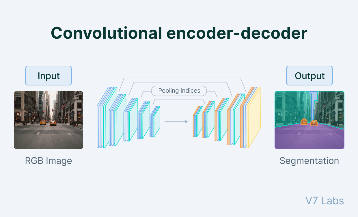
In the encoder part of the network, we go from a large image to small matrix. That small matrix contains the semantic information describing the image. We effectively embed the image as that small matrix.

Embedding words

Embedding a word is pretty much the same idea. The natwork wants to store that symbol as a vector and the direction of the vector encodes some semantic information about the word.

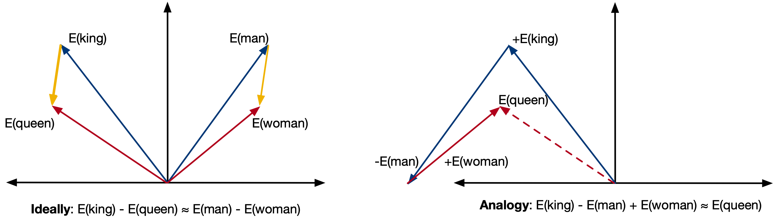
What's interesting is that if the embedding is done well, the relative position between embeddings is itself a embedding and contains some semantic information! We can see this is code by analyzing one of the OG embedding schemes GLoVe embeddings:

import gensim.downloader
import numpy as np
from sklearn.metrics.pairwise import cosine_similarity

# Load the GloVe 50-dimensional model
model = gensim.downloader.load("glove-wiki-gigaword-50")

# 1. Basic embedding lookup
word = "tower"
vector = model[word]
print(f"Embedding for '{word}':\n{vector}\n")

# 2. Embedding math: analogy task (king - man + woman ≈ queen)
result_vector = model["king"] - model["man"] + model["woman"]

# Find closest word to result_vector
similar_words = model.similar_by_vector(result_vector, topn=5)
print("Closest words to 'king - man + woman':")
for word, similarity in similar_words:
    print(f"  {word}: {similarity:.3f}")

print()

# 3. Cosine similarity between two words
def cosine_sim(w1, w2):
    v1 = model[w1].reshape(1, -1)
    v2 = model[w2].reshape(1, -1)
    return cosine_similarity(v1, v2)[0][0]

sim = cosine_sim("king", "queen")
print(f"Cosine similarity between 'king' and 'queen': {sim:.3f}")

sim2 = cosine_sim("tower", "building")
print(f"Cosine similarity between 'tower' and 'building': {sim2:.3f}")

print()

# 4. Create a custom vector (mix two concepts) and find nearby words
custom_vector = (model["river"] + model["mountain"]) / 2
similar_words = model.similar_by_vector(custom_vector, topn=5)
print("Words similar to average of 'river' and 'mountain':")
for word, similarity in similar_words:
    print(f"  {word}: {similarity:.3f}")

[=============================---------------------] 58.4% 38.5/66.0MB downloaded

IOPub message rate exceeded.
The notebook server will temporarily stop sending output
to the client in order to avoid crashing it.
To change this limit, set the config variable
`--NotebookApp.iopub_msg_rate_limit`.

Current values:
NotebookApp.iopub_msg_rate_limit=1000.0 (msgs/sec)
NotebookApp.rate_limit_window=3.0 (secs)

[==================================================] 100.0% 66.0/66.0MB downloaded
Embedding for 'tower':
[ 1.1474e+00  1.1811e+00  7.4556e-01 -5.9101e-02  5.0499e-01 -7.0449e-01
 -3.2136e-01 -4.5390e-01 -4.5763e-01 -7.5341e-01 -3.3511e-01 -2.4975e-02
 -5.0192e-01  6.3773e-01 -8.3059e-01  8.3565e-01 -2.4701e-01  3.2421e-01
 -1.1103e+00 -2.1335e-02  6.8717e-01 -3.9340e-01 -1.6390e+00 -5.0493e-01
 -1.6684e-01 -6.7649e-01 -3.1798e-01  8.8503e-01 -3.1552e-02 -1.5608e-01
  1.9805e+00 -1.1870e+00  8.3342e-01 -1.8369e-01 -2.6691e-01  1.1619e-01
  1.1023e+00 -3.5937e-01  2.5015e-02 -4.0615e-02  3.0681e-01 -4.1076e-01
  8.4586e-02  2.2475e-01 -5.0955e-01  6.5819e-01 -1.2432e-01 -1.4039e+00
  1.6178e-04 -5.2529e-01]

Closest words to 'king - man + woman':
  king: 0.886
  queen: 0.861
  daughter: 0.768
  prince: 0.764
  throne: 0.763

Cosine similarity between 'king' and 'queen': 0.784
Cosine similarity between 'tower' and 'building': 0.787

Words similar to average of 'river' and 'mountain':
  river: 0.932
  mountain: 0.898
  valley: 0.896
  mountains: 0.858
  creek: 0.846

The important thing to remember is that computer accepts numbers, not symbols. So let's assume word tokenization. We need to embed the words as n-dimensional vectors.

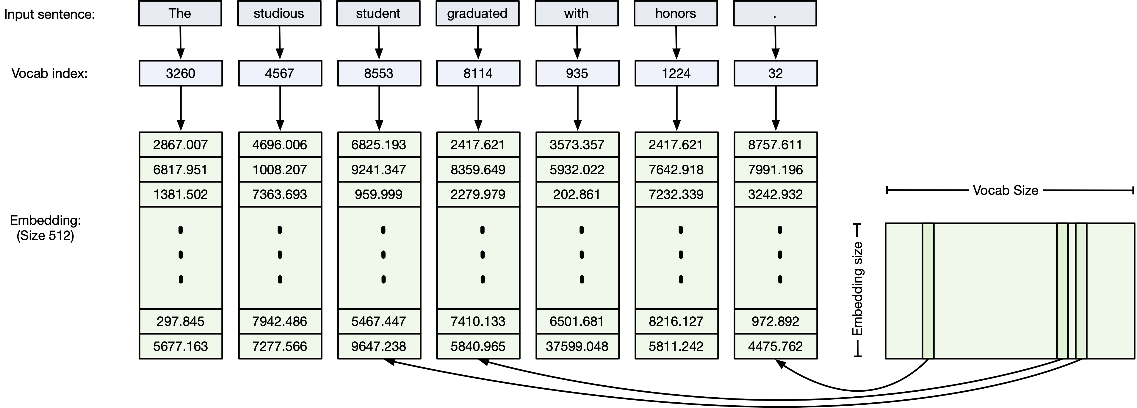
• remember, the embedding matrix is trainable. Just another set of parameters that needs to be train of thousands of iterations on large datasets

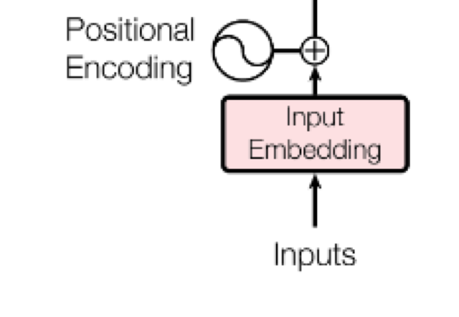
Step 2: Positional encoding

Core concept: We want to give the model a method to reference a word at a particular positon in the sentence.

Some nuances:

• We want each word to carry information about its position in the sentence
• We want words that are close together to have similar positional encodings and the words that are far apart to have dissimilar position encodings.
• Needs to be something that the model can learn.
• Would be nice to only encode the encodings once (so no variable encodings for each sentence)

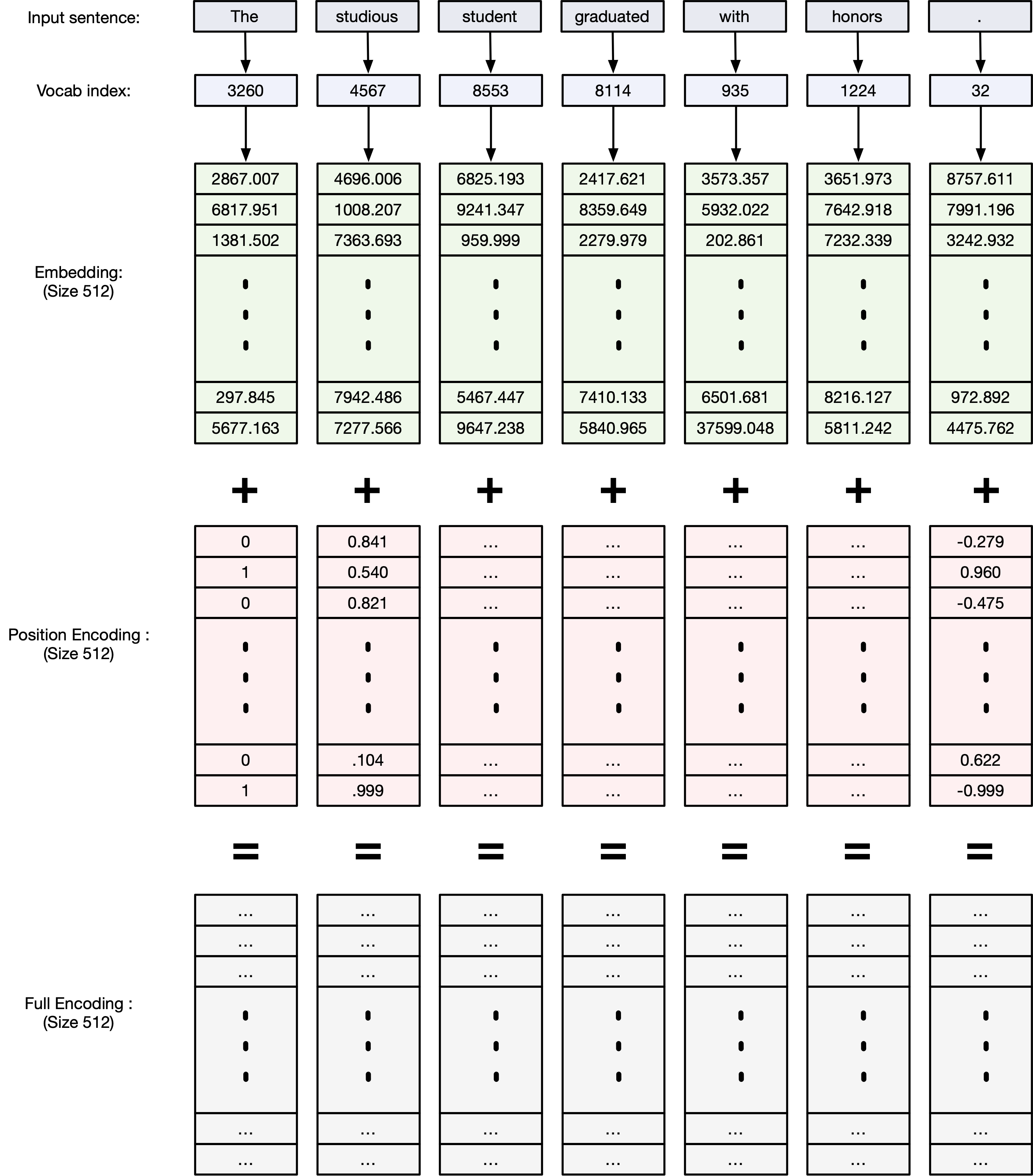
Sinusoidal Positional Encoding - (Vaswani et al., 2017)

In the original Transformer paper ("Attention is All You Need"), fixed sinusoidal functions were used:

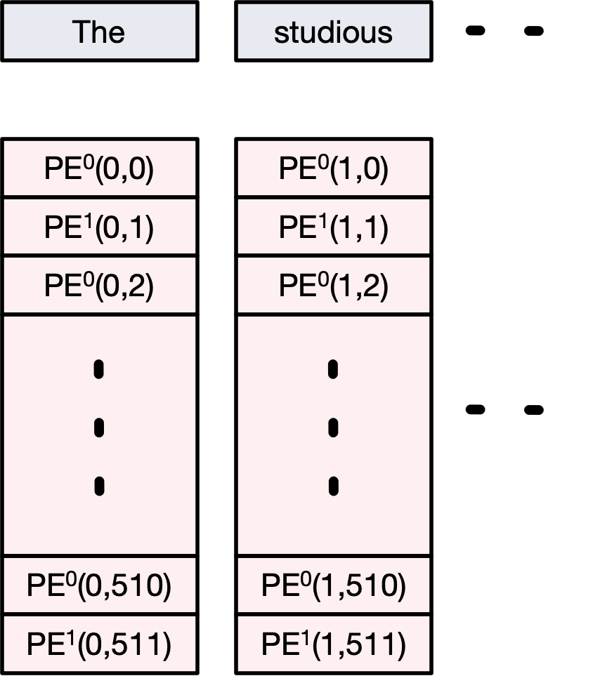
For a position $pos$ and dimension $i$, the encoding is defined as:

$$ \text{PE}^0_{(pos, 2i)} = \sin\left(\frac{pos}{10000^{2i/d_{\text{model}}}}\right) $$$$ \text{PE}^1_{(pos, 2i+1)} = \cos\left(\frac{pos}{10000^{2i/d_{\text{model}}}}\right) $$

Where:

• $pos$ = position in the sequence
• $i$ = embedding dimension index
• $d_{\text{model}}$ = total embedding size (e.g., 512)

Even dimensions → sine
Odd dimensions → cosine

Intuition:

• Different frequencies allow each position to be uniquely encoded.
• Nearby positions have similar encodings (smooth changes).
• Generalizes to sequences longer than what the model was trained on.

Conceptual explanation

I found a blog post that gives the best explanation so far about why the positonal encodings are formulated the way they are. Here's the cliff notes:

We need a positional encoding that satisfies the realtive criteria:

• It should output a unique encoding for each time-step (word’s position in a sentence)
• Distance between any two time-steps should be consistent across sentences with different lengths.
• Our model should generalize to longer sentences without any efforts. Its values should be bounded.
• It must be deterministic.

Why sines and cosines?

Suppose we want to represent a number in binary format:

	Bit 3	Bit 2	Bit 1	Bit 0		Bit 3	Bit 2	Bit 1	Bit 0
0	0	0	0	0	8	1	0	0	0
1	0	0	0	1	9	1	0	0	1
2	0	0	1	0	10	1	0	1	0
3	0	0	1	1	11	1	0	1	1
4	0	1	0	0	12	1	1	0	0
5	0	1	0	1	13	1	1	0	1
6	0	1	1	0	14	1	1	1	0
7	0	1	1	1	15	1	1	1	1

Each bit position has a different frequency. That is pretty much what we're doing with the positonal vectors above representng the dimension and pos as frequencies.

Relative positioning

The other benefit is that we can calculate relative postioning fairly easily:

$$ M \cdot \begin{bmatrix} \sin(\omega_k t) \\ \cos(\omega_k t) \end{bmatrix} = \begin{bmatrix} \sin(\omega_k (t + \phi)) \\ \cos(\omega_k (t + \phi)) \end{bmatrix} $$

---

Proof:

Let $M$ be a $2 \times 2$ matrix, we want to find $u_1, v_1, u_2$ and $v_2$ so that:

$$ \begin{bmatrix} u_1 & v_1 \\ u_2 & v_2 \end{bmatrix} \cdot \begin{bmatrix} \sin(\omega_k t) \\ \cos(\omega_k t) \end{bmatrix} = \begin{bmatrix} \sin(\omega_k (t + \phi)) \\ \cos(\omega_k (t + \phi)) \end{bmatrix} $$

By applying the addition theorem, we can expand the right-hand side as follows:

$$ \begin{bmatrix} u_1 & v_1 \\ u_2 & v_2 \end{bmatrix} \cdot \begin{bmatrix} \sin(\omega_k t) \\ \cos(\omega_k t) \end{bmatrix} = \begin{bmatrix} \sin(\omega_k t) \cos(\omega_k \phi) + \cos(\omega_k t) \sin(\omega_k \phi) \\ \cos(\omega_k t) \cos(\omega_k \phi) - \sin(\omega_k t) \sin(\omega_k \phi) \end{bmatrix} $$

Which results in the following two equations:

$$ u_1 \sin(\omega_k t) + v_1 \cos(\omega_k t) = \cos(\omega_k \phi) \sin(\omega_k t) + \sin(\omega_k \phi) \cos(\omega_k t) \tag{1} $$$$ u_2 \sin(\omega_k t) + v_2 \cos(\omega_k t) = -\sin(\omega_k \phi) \sin(\omega_k t) + \cos(\omega_k \phi) \cos(\omega_k t) \tag{2} $$

By solving the above equations, we get:

$$ u_1 = \cos(\omega_k \phi) \quad v_1 = \sin(\omega_k \phi) $$$$ u_2 = -\sin(\omega_k \phi) \quad v_2 = \cos(\omega_k \phi) $$

---

Thus, the final transformation matrix $M$ is:

$$ M_{\phi,k} = \begin{bmatrix} \cos(\omega_k \phi) & \sin(\omega_k \phi) \\ -\sin(\omega_k \phi) & \cos(\omega_k \phi) \end{bmatrix} $$

This is likely why sine/cosine are both used. There isn't a clear linear transformation with only sine or only cosine.

import numpy as np
import matplotlib.pyplot as plt

def plot_positional_encoding(seq_len=100, d_model=64, save_path=None):
    """
    Plots the positional encoding and optionally saves the figure.
    
    Args:
        seq_len (int): Number of positions (x-axis).
        d_model (int): Embedding depth (y-axis).
        save_path (str, optional): If provided, saves the figure to this path.
    """
    def get_sinusoidal_encoding(seq_len, d_model):
        pos = np.arange(seq_len)[:, None]
        i = np.arange(d_model)[None, :]
        angle_rates = 1 / np.power(10000, (2 * (i // 2)) / d_model)
        angle_rads = pos * angle_rates

        pos_encoding = np.zeros(angle_rads.shape)
        pos_encoding[:, 0::2] = np.sin(angle_rads[:, 0::2])
        pos_encoding[:, 1::2] = np.cos(angle_rads[:, 1::2])

        return pos_encoding

    pos_encoding = get_sinusoidal_encoding(seq_len, d_model)

    plt.figure(figsize=(8, 6))
    plt.imshow(pos_encoding.T, aspect='auto', cmap='viridis', origin='lower')
    plt.colorbar(label='Encoding Value')
    plt.xlabel('Position')
    plt.ylabel('Depth (Embedding Dimension)')
    plt.title('Positional Encoding (Sinusoidal)')
    plt.tight_layout()
    
    if save_path:
        plt.savefig(save_path, dpi=300)
        print(f"Figure saved to {save_path}")
    else:
        plt.show()

# Example usage:
plot_positional_encoding(seq_len=100, d_model=64, save_path=None)  # Show figure
# plot_positional_encoding(seq_len=100, d_model=64, save_path='positional_encoding.png')  # Save figure

Why is Positional Encoding a Function of Sin/Cos?

When designing the Transformer (Vaswani et al., 2017), the key challenge was:

Transformers have no recurrence and no convolution — how do we tell the model the order of tokens?

Core Reasons for Using Sinusoids

1. Captures Relative and Absolute Position

• Sinusoids are smooth and periodic.
• They encode both:
  • Absolute position: Each position gets a unique vector.
  • Relative distance: Easy to infer how far apart two positions are.

Note: $$ \sin(a + b) = \sin(a)\cos(b) + \cos(a)\sin(b) $$ Thus, the model can easily compute relative offsets based on the sin/cos values.

2. No Extra Parameters

• Sinusoidal functions are fixed — no extra weights to learn.
• Transformer can extrapolate to longer sequences during inference without retraining.

3. Multi-Scale Representations

• Different dimensions have different frequencies:
  • Low-frequency sinusoids capture long-range patterns.
  • High-frequency sinusoids capture local patterns.

"We use sine and cosine functions of different frequencies. For each position, we generate a vector whose even indices are sine functions and whose odd indices are cosine functions of different wavelengths."

This lets the model attend both to nearby and distant tokens effectively.

---

There are other position encoding schemes [5]:

"There are many choices of positional encodings, learned and fixed ... We also experimented with using learned positional embeddings instead, and found that the two versions produced nearly identical results"

That's it for today

• Next time we'll discuss attention
• HW10 (last HW!) will be released tomorrow
• And most importantly, have a good weekend.

References

[1] Bengio, Yoshua, Patrice Simard, and Paolo Frasconi. "Learning long-term dependencies with gradient descent is difficult." IEEE transactions on neural networks 5.2 (1994): 157-166.

[2] Vaswani, Ashish, et al. "Attention is all you need." Advances in neural information processing systems 30 (2017).

[3] Umar Jamil "Attention is all you need (Transformer) - Model explanation (including math), Inference and Training" - https://www.youtube.com/watch?v=bCz4OMemCcA

[4] 3Blue1Brown "Attention in transformers, step-by-step | DL6" https://www.youtube.com/watch?v=eMlx5fFNoYc

[5] Adrian Tam, "Positional Encodings in Transformer Models" https://machinelearningmastery.com/positional-encodings-in-transformer-models/