Things we'll cover in today's lecture:
- More matrix operations
- Solving systems of linear equations
- Eigen decomposition of symmetric matrices
More matrix operations
Here are more functions for matrix operations:
Slice:
- Slicing means selecting the elements present in the tensor by using “:” slice operator. We can slice the elements by using the index of that particular element.
- Let’s create a 3D Tensor for demonstration. We can create a vector by using torch.tensor() function
# import torch module
import torch

# create an 3 D tensor with 8 elements each
a = torch.tensor([[[1, 2, 3, 4, 5, 6, 7, 8],
                   [10, 11, 12, 13, 14, 15, 16, 17]],

                  [[71, 72, 73, 74, 75, 76, 77, 78],
                   [81, 82, 83, 84, 85, 86, 87, 88]]])

# display actual  tensor
print(a)
tensor([[[ 1,  2,  3,  4,  5,  6,  7,  8],
         [10, 11, 12, 13, 14, 15, 16, 17]],

        [[71, 72, 73, 74, 75, 76, 77, 78],
         [81, 82, 83, 84, 85, 86, 87, 88]]])
Alertness Check: What is the shape of this tensor?
print(a.shape)
Alertness Check: Some fun slicing problems:
a = torch.tensor([[[1, 2, 3, 4, 5, 6, 7, 8],
                   [10, 11, 12, 13, 14, 15, 16, 17]],

                  [[71, 72, 73, 74, 75, 76, 77, 78],
                   [81, 82, 83, 84, 85, 86, 87, 88]]])

# display actual  tensor
print(a)
tensor([[[ 1,  2,  3,  4,  5,  6,  7,  8],
         [10, 11, 12, 13, 14, 15, 16, 17]],

        [[71, 72, 73, 74, 75, 76, 77, 78],
         [81, 82, 83, 84, 85, 86, 87, 88]]])
How do we get every other value in the first row displayed above?
# access  all the tensors of 1
# dimension and get only 7 values
# in that dimension
print(a[0:1, 0:1, :8:2])
tensor([[[1, 3, 5, 7]]])
a = torch.tensor([[[1, 2, 3, 4, 5, 6, 7, 8],
                   [10, 11, 12, 13, 14, 15, 16, 17]],

                  [[71, 72, 73, 74, 75, 76, 77, 78],
                   [81, 82, 83, 84, 85, 86, 87, 88]]])

# display actual  tensor
print(a)
tensor([[[ 1,  2,  3,  4,  5,  6,  7,  8],
         [10, 11, 12, 13, 14, 15, 16, 17]],

        [[71, 72, 73, 74, 75, 76, 77, 78],
         [81, 82, 83, 84, 85, 86, 87, 88]]])
What will the code below display (value and shape)?
# access  all the tensors of all
# dimensions and get only 3 values
# in each dimension
print(a[0:1, 0:2, :3])
a = torch.tensor([[[1, 2, 3, 4, 5, 6, 7, 8],
                   [10, 11, 12, 13, 14, 15, 16, 17]],

                  [[71, 72, 73, 74, 75, 76, 77, 78],
                   [81, 82, 83, 84, 85, 86, 87, 88]]])

# display actual  tensor
print(a)
tensor([[[ 1,  2,  3,  4,  5,  6,  7,  8],
         [10, 11, 12, 13, 14, 15, 16, 17]],

        [[71, 72, 73, 74, 75, 76, 77, 78],
         [81, 82, 83, 84, 85, 86, 87, 88]]])
What will the code below display (value and shape)?
# access 8 elements in 1 dimension
# on all tensors
print(a[0:2, 1, 0:8])
Broadcasting
Quick diversion, what is the output of the following code:
import torch

a = torch.arange(2).view(-1,1)
b = torch.arange(2).view(1,-1)

print(a+b)
import numpy as np

a = np.array([0, 1])
b = np.array([[0], [1]])

print(a+b)
[[0 1]
 [1 2]]
While everyone is familiar with numpy(torch) slicing, broadcasting it less used. So I thought it would be worthwhile to brush upon it quickly.
When adding a array and a scaler, we know we want to add the element to every element in the array.
import numpy as np

a = np.array([1,2,3,4])
b = a+1

print(b)
[2 3 4 5]
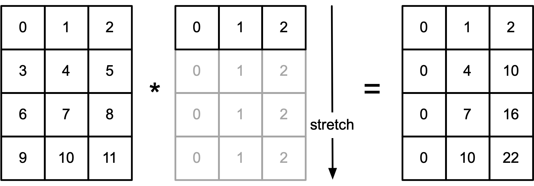
Another way to look at this is that the dimension of b is being stretched:

Works with matrix to matrix operations too:
import torch

a = torch.arange(12).view(4,3)
b = torch.arange(3).view(1,3)

print(a)
print(b)
print(a*b)
tensor([[ 0,  1,  2],
        [ 3,  4,  5],
        [ 6,  7,  8],
        [ 9, 10, 11]])
tensor([[0, 1, 2]])
tensor([[ 0,  1,  4],
        [ 0,  4, 10],
        [ 0,  7, 16],
        [ 0, 10, 22]])
General broadcasting rule:
When operating two arrays, NumPy compares their shapes, element-wise from right to left and tries to find two dimensions that are:
- equal
- one of them is size 1
Then it stretches those dimenisons to make the array match.
Two arrays do not need to have to same number of dimenisons, but the resulting array will have the number of dimenisons equal to the input array with the greatest number of dimensions.
What does the following code snippet produce:
import torch

a = torch.tensor([[0,1,2,3], [4,5,6,7]])
b = torch.tensor([[0,1,2]])

print(a)
print(b)
print(a*b)
Broadasting provides a useful way fo taking the outer-product of any set of arrays
import torch

# Define the size of each dimension
size = 10

# Create the 4D array with shape (10, 10, 10, 10)
# Generate indices from 0 to 9 in each dimension
a = torch.arange(size).view(-1, 1, 1, 1)  # Shape (10, 1, 1, 1)
b = torch.arange(size).view(1, -1, 1, 1)  # Shape (1, 10, 1, 1)
c = torch.arange(size).view(1, 1, -1, 1)  # Shape (1, 1, 10, 1)
d = torch.arange(size).view(1, 1, 1, -1)  # Shape (1, 1, 1, 10)

# Compute the 4D array where each index corresponds to the concatenation of a, b, c, d
x = a * 1000 + b * 100 + c * 10 + d

# Print the resulting 4D tensor
print(x)
tensor([[[[   0,    1,    2,  ...,    7,    8,    9],
          [  10,   11,   12,  ...,   17,   18,   19],
          [  20,   21,   22,  ...,   27,   28,   29],
          ...,
          [  70,   71,   72,  ...,   77,   78,   79],
          [  80,   81,   82,  ...,   87,   88,   89],
          [  90,   91,   92,  ...,   97,   98,   99]],

         [[ 100,  101,  102,  ...,  107,  108,  109],
          [ 110,  111,  112,  ...,  117,  118,  119],
          [ 120,  121,  122,  ...,  127,  128,  129],
          ...,
          [ 170,  171,  172,  ...,  177,  178,  179],
          [ 180,  181,  182,  ...,  187,  188,  189],
          [ 190,  191,  192,  ...,  197,  198,  199]],

         [[ 200,  201,  202,  ...,  207,  208,  209],
          [ 210,  211,  212,  ...,  217,  218,  219],
          [ 220,  221,  222,  ...,  227,  228,  229],
          ...,
          [ 270,  271,  272,  ...,  277,  278,  279],
          [ 280,  281,  282,  ...,  287,  288,  289],
          [ 290,  291,  292,  ...,  297,  298,  299]],

         ...,

         [[ 700,  701,  702,  ...,  707,  708,  709],
          [ 710,  711,  712,  ...,  717,  718,  719],
          [ 720,  721,  722,  ...,  727,  728,  729],
          ...,
          [ 770,  771,  772,  ...,  777,  778,  779],
          [ 780,  781,  782,  ...,  787,  788,  789],
          [ 790,  791,  792,  ...,  797,  798,  799]],

         [[ 800,  801,  802,  ...,  807,  808,  809],
          [ 810,  811,  812,  ...,  817,  818,  819],
          [ 820,  821,  822,  ...,  827,  828,  829],
          ...,
          [ 870,  871,  872,  ...,  877,  878,  879],
          [ 880,  881,  882,  ...,  887,  888,  889],
          [ 890,  891,  892,  ...,  897,  898,  899]],

         [[ 900,  901,  902,  ...,  907,  908,  909],
          [ 910,  911,  912,  ...,  917,  918,  919],
          [ 920,  921,  922,  ...,  927,  928,  929],
          ...,
          [ 970,  971,  972,  ...,  977,  978,  979],
          [ 980,  981,  982,  ...,  987,  988,  989],
          [ 990,  991,  992,  ...,  997,  998,  999]]],


        [[[1000, 1001, 1002,  ..., 1007, 1008, 1009],
          [1010, 1011, 1012,  ..., 1017, 1018, 1019],
          [1020, 1021, 1022,  ..., 1027, 1028, 1029],
          ...,
          [1070, 1071, 1072,  ..., 1077, 1078, 1079],
          [1080, 1081, 1082,  ..., 1087, 1088, 1089],
          [1090, 1091, 1092,  ..., 1097, 1098, 1099]],

         [[1100, 1101, 1102,  ..., 1107, 1108, 1109],
          [1110, 1111, 1112,  ..., 1117, 1118, 1119],
          [1120, 1121, 1122,  ..., 1127, 1128, 1129],
          ...,
          [1170, 1171, 1172,  ..., 1177, 1178, 1179],
          [1180, 1181, 1182,  ..., 1187, 1188, 1189],
          [1190, 1191, 1192,  ..., 1197, 1198, 1199]],

         [[1200, 1201, 1202,  ..., 1207, 1208, 1209],
          [1210, 1211, 1212,  ..., 1217, 1218, 1219],
          [1220, 1221, 1222,  ..., 1227, 1228, 1229],
          ...,
          [1270, 1271, 1272,  ..., 1277, 1278, 1279],
          [1280, 1281, 1282,  ..., 1287, 1288, 1289],
          [1290, 1291, 1292,  ..., 1297, 1298, 1299]],

         ...,

         [[1700, 1701, 1702,  ..., 1707, 1708, 1709],
          [1710, 1711, 1712,  ..., 1717, 1718, 1719],
          [1720, 1721, 1722,  ..., 1727, 1728, 1729],
          ...,
          [1770, 1771, 1772,  ..., 1777, 1778, 1779],
          [1780, 1781, 1782,  ..., 1787, 1788, 1789],
          [1790, 1791, 1792,  ..., 1797, 1798, 1799]],

         [[1800, 1801, 1802,  ..., 1807, 1808, 1809],
          [1810, 1811, 1812,  ..., 1817, 1818, 1819],
          [1820, 1821, 1822,  ..., 1827, 1828, 1829],
          ...,
          [1870, 1871, 1872,  ..., 1877, 1878, 1879],
          [1880, 1881, 1882,  ..., 1887, 1888, 1889],
          [1890, 1891, 1892,  ..., 1897, 1898, 1899]],

         [[1900, 1901, 1902,  ..., 1907, 1908, 1909],
          [1910, 1911, 1912,  ..., 1917, 1918, 1919],
          [1920, 1921, 1922,  ..., 1927, 1928, 1929],
          ...,
          [1970, 1971, 1972,  ..., 1977, 1978, 1979],
          [1980, 1981, 1982,  ..., 1987, 1988, 1989],
          [1990, 1991, 1992,  ..., 1997, 1998, 1999]]],


        [[[2000, 2001, 2002,  ..., 2007, 2008, 2009],
          [2010, 2011, 2012,  ..., 2017, 2018, 2019],
          [2020, 2021, 2022,  ..., 2027, 2028, 2029],
          ...,
          [2070, 2071, 2072,  ..., 2077, 2078, 2079],
          [2080, 2081, 2082,  ..., 2087, 2088, 2089],
          [2090, 2091, 2092,  ..., 2097, 2098, 2099]],

         [[2100, 2101, 2102,  ..., 2107, 2108, 2109],
          [2110, 2111, 2112,  ..., 2117, 2118, 2119],
          [2120, 2121, 2122,  ..., 2127, 2128, 2129],
          ...,
          [2170, 2171, 2172,  ..., 2177, 2178, 2179],
          [2180, 2181, 2182,  ..., 2187, 2188, 2189],
          [2190, 2191, 2192,  ..., 2197, 2198, 2199]],

         [[2200, 2201, 2202,  ..., 2207, 2208, 2209],
          [2210, 2211, 2212,  ..., 2217, 2218, 2219],
          [2220, 2221, 2222,  ..., 2227, 2228, 2229],
          ...,
          [2270, 2271, 2272,  ..., 2277, 2278, 2279],
          [2280, 2281, 2282,  ..., 2287, 2288, 2289],
          [2290, 2291, 2292,  ..., 2297, 2298, 2299]],

         ...,

         [[2700, 2701, 2702,  ..., 2707, 2708, 2709],
          [2710, 2711, 2712,  ..., 2717, 2718, 2719],
          [2720, 2721, 2722,  ..., 2727, 2728, 2729],
          ...,
          [2770, 2771, 2772,  ..., 2777, 2778, 2779],
          [2780, 2781, 2782,  ..., 2787, 2788, 2789],
          [2790, 2791, 2792,  ..., 2797, 2798, 2799]],

         [[2800, 2801, 2802,  ..., 2807, 2808, 2809],
          [2810, 2811, 2812,  ..., 2817, 2818, 2819],
          [2820, 2821, 2822,  ..., 2827, 2828, 2829],
          ...,
          [2870, 2871, 2872,  ..., 2877, 2878, 2879],
          [2880, 2881, 2882,  ..., 2887, 2888, 2889],
          [2890, 2891, 2892,  ..., 2897, 2898, 2899]],

         [[2900, 2901, 2902,  ..., 2907, 2908, 2909],
          [2910, 2911, 2912,  ..., 2917, 2918, 2919],
          [2920, 2921, 2922,  ..., 2927, 2928, 2929],
          ...,
          [2970, 2971, 2972,  ..., 2977, 2978, 2979],
          [2980, 2981, 2982,  ..., 2987, 2988, 2989],
          [2990, 2991, 2992,  ..., 2997, 2998, 2999]]],


        ...,


        [[[7000, 7001, 7002,  ..., 7007, 7008, 7009],
          [7010, 7011, 7012,  ..., 7017, 7018, 7019],
          [7020, 7021, 7022,  ..., 7027, 7028, 7029],
          ...,
          [7070, 7071, 7072,  ..., 7077, 7078, 7079],
          [7080, 7081, 7082,  ..., 7087, 7088, 7089],
          [7090, 7091, 7092,  ..., 7097, 7098, 7099]],

         [[7100, 7101, 7102,  ..., 7107, 7108, 7109],
          [7110, 7111, 7112,  ..., 7117, 7118, 7119],
          [7120, 7121, 7122,  ..., 7127, 7128, 7129],
          ...,
          [7170, 7171, 7172,  ..., 7177, 7178, 7179],
          [7180, 7181, 7182,  ..., 7187, 7188, 7189],
          [7190, 7191, 7192,  ..., 7197, 7198, 7199]],

         [[7200, 7201, 7202,  ..., 7207, 7208, 7209],
          [7210, 7211, 7212,  ..., 7217, 7218, 7219],
          [7220, 7221, 7222,  ..., 7227, 7228, 7229],
          ...,
          [7270, 7271, 7272,  ..., 7277, 7278, 7279],
          [7280, 7281, 7282,  ..., 7287, 7288, 7289],
          [7290, 7291, 7292,  ..., 7297, 7298, 7299]],

         ...,

         [[7700, 7701, 7702,  ..., 7707, 7708, 7709],
          [7710, 7711, 7712,  ..., 7717, 7718, 7719],
          [7720, 7721, 7722,  ..., 7727, 7728, 7729],
          ...,
          [7770, 7771, 7772,  ..., 7777, 7778, 7779],
          [7780, 7781, 7782,  ..., 7787, 7788, 7789],
          [7790, 7791, 7792,  ..., 7797, 7798, 7799]],

         [[7800, 7801, 7802,  ..., 7807, 7808, 7809],
          [7810, 7811, 7812,  ..., 7817, 7818, 7819],
          [7820, 7821, 7822,  ..., 7827, 7828, 7829],
          ...,
          [7870, 7871, 7872,  ..., 7877, 7878, 7879],
          [7880, 7881, 7882,  ..., 7887, 7888, 7889],
          [7890, 7891, 7892,  ..., 7897, 7898, 7899]],

         [[7900, 7901, 7902,  ..., 7907, 7908, 7909],
          [7910, 7911, 7912,  ..., 7917, 7918, 7919],
          [7920, 7921, 7922,  ..., 7927, 7928, 7929],
          ...,
          [7970, 7971, 7972,  ..., 7977, 7978, 7979],
          [7980, 7981, 7982,  ..., 7987, 7988, 7989],
          [7990, 7991, 7992,  ..., 7997, 7998, 7999]]],


        [[[8000, 8001, 8002,  ..., 8007, 8008, 8009],
          [8010, 8011, 8012,  ..., 8017, 8018, 8019],
          [8020, 8021, 8022,  ..., 8027, 8028, 8029],
          ...,
          [8070, 8071, 8072,  ..., 8077, 8078, 8079],
          [8080, 8081, 8082,  ..., 8087, 8088, 8089],
          [8090, 8091, 8092,  ..., 8097, 8098, 8099]],

         [[8100, 8101, 8102,  ..., 8107, 8108, 8109],
          [8110, 8111, 8112,  ..., 8117, 8118, 8119],
          [8120, 8121, 8122,  ..., 8127, 8128, 8129],
          ...,
          [8170, 8171, 8172,  ..., 8177, 8178, 8179],
          [8180, 8181, 8182,  ..., 8187, 8188, 8189],
          [8190, 8191, 8192,  ..., 8197, 8198, 8199]],

         [[8200, 8201, 8202,  ..., 8207, 8208, 8209],
          [8210, 8211, 8212,  ..., 8217, 8218, 8219],
          [8220, 8221, 8222,  ..., 8227, 8228, 8229],
          ...,
          [8270, 8271, 8272,  ..., 8277, 8278, 8279],
          [8280, 8281, 8282,  ..., 8287, 8288, 8289],
          [8290, 8291, 8292,  ..., 8297, 8298, 8299]],

         ...,

         [[8700, 8701, 8702,  ..., 8707, 8708, 8709],
          [8710, 8711, 8712,  ..., 8717, 8718, 8719],
          [8720, 8721, 8722,  ..., 8727, 8728, 8729],
          ...,
          [8770, 8771, 8772,  ..., 8777, 8778, 8779],
          [8780, 8781, 8782,  ..., 8787, 8788, 8789],
          [8790, 8791, 8792,  ..., 8797, 8798, 8799]],

         [[8800, 8801, 8802,  ..., 8807, 8808, 8809],
          [8810, 8811, 8812,  ..., 8817, 8818, 8819],
          [8820, 8821, 8822,  ..., 8827, 8828, 8829],
          ...,
          [8870, 8871, 8872,  ..., 8877, 8878, 8879],
          [8880, 8881, 8882,  ..., 8887, 8888, 8889],
          [8890, 8891, 8892,  ..., 8897, 8898, 8899]],

         [[8900, 8901, 8902,  ..., 8907, 8908, 8909],
          [8910, 8911, 8912,  ..., 8917, 8918, 8919],
          [8920, 8921, 8922,  ..., 8927, 8928, 8929],
          ...,
          [8970, 8971, 8972,  ..., 8977, 8978, 8979],
          [8980, 8981, 8982,  ..., 8987, 8988, 8989],
          [8990, 8991, 8992,  ..., 8997, 8998, 8999]]],


        [[[9000, 9001, 9002,  ..., 9007, 9008, 9009],
          [9010, 9011, 9012,  ..., 9017, 9018, 9019],
          [9020, 9021, 9022,  ..., 9027, 9028, 9029],
          ...,
          [9070, 9071, 9072,  ..., 9077, 9078, 9079],
          [9080, 9081, 9082,  ..., 9087, 9088, 9089],
          [9090, 9091, 9092,  ..., 9097, 9098, 9099]],

         [[9100, 9101, 9102,  ..., 9107, 9108, 9109],
          [9110, 9111, 9112,  ..., 9117, 9118, 9119],
          [9120, 9121, 9122,  ..., 9127, 9128, 9129],
          ...,
          [9170, 9171, 9172,  ..., 9177, 9178, 9179],
          [9180, 9181, 9182,  ..., 9187, 9188, 9189],
          [9190, 9191, 9192,  ..., 9197, 9198, 9199]],

         [[9200, 9201, 9202,  ..., 9207, 9208, 9209],
          [9210, 9211, 9212,  ..., 9217, 9218, 9219],
          [9220, 9221, 9222,  ..., 9227, 9228, 9229],
          ...,
          [9270, 9271, 9272,  ..., 9277, 9278, 9279],
          [9280, 9281, 9282,  ..., 9287, 9288, 9289],
          [9290, 9291, 9292,  ..., 9297, 9298, 9299]],

         ...,

         [[9700, 9701, 9702,  ..., 9707, 9708, 9709],
          [9710, 9711, 9712,  ..., 9717, 9718, 9719],
          [9720, 9721, 9722,  ..., 9727, 9728, 9729],
          ...,
          [9770, 9771, 9772,  ..., 9777, 9778, 9779],
          [9780, 9781, 9782,  ..., 9787, 9788, 9789],
          [9790, 9791, 9792,  ..., 9797, 9798, 9799]],

         [[9800, 9801, 9802,  ..., 9807, 9808, 9809],
          [9810, 9811, 9812,  ..., 9817, 9818, 9819],
          [9820, 9821, 9822,  ..., 9827, 9828, 9829],
          ...,
          [9870, 9871, 9872,  ..., 9877, 9878, 9879],
          [9880, 9881, 9882,  ..., 9887, 9888, 9889],
          [9890, 9891, 9892,  ..., 9897, 9898, 9899]],

         [[9900, 9901, 9902,  ..., 9907, 9908, 9909],
          [9910, 9911, 9912,  ..., 9917, 9918, 9919],
          [9920, 9921, 9922,  ..., 9927, 9928, 9929],
          ...,
          [9970, 9971, 9972,  ..., 9977, 9978, 9979],
          [9980, 9981, 9982,  ..., 9987, 9988, 9989],
          [9990, 9991, 9992,  ..., 9997, 9998, 9999]]]])
Linear equations
What is a linear equation?
- Wikipedia defines a system of linear equations as:
In mathematics, a system of linear equations (or linear system) is a collection of two or more linear equations involving the same set of variables.
Representing Systems of Linear Equations using Matrices
- A system of linear equations can be represented in matrix form using a coefficient matrix, a variable matrix, and a constant matrix.
- General form of a linear system: A linear system has $n$ unknown and $m$ equations:
$\begin{array}{c}
a_{11}x_{1}+a_{12}x_{2}+\ldots+a_{1n}x_{n}=b_{1}\ a_{21}x_{1}+a_{22}x_{2}+\ldots+a_{2n}x_{n}=b_{2}\ \vdots\ a_{m1}x_{1}+a_{m2}x_{2}+\ldots+a_{mn}x_{n}=b_{m} \end{array}$ <Br> Where $x_1, x_2,..., x_n$ are the unknowns, $a_11, a_12, ..., a_mn$ are the coefficients of the system, and $b_1, b_2,..., b_m$ are the constant terms.
- Vector equation: One helpful view is that each unknown is a weight for a column vector in a linear combination
$x_{1}\left[\begin{array}{c} a_{11}\\ a_{21}\\ \vdots\\ a_{m1} \end{array}\right]+x_{2}\left[\begin{array}{c} a_{12}\\ a_{22}\\ \vdots\\ a_{m2} \end{array}\right]+\cdots+x_{n}\left[\begin{array}{c} a_{1n}\\ a_{2n}\\ \vdots\\ a_{mn} \end{array}\right]=\left[\begin{array}{c} b_{1}\\ b_{2}\\ \vdots\\ b_{m} \end{array}\right]$
Representing Systems of Linear Equations using Matrices
Matrix equation: The vector equation is equivalent to a matrix equation of the form.
$Ax=\left[\begin{matrix}a_{11} & a_{12} & \ldots & a_{1n}\
a_{21} & a_{22} & \vdots & a_{2n}\
\vdots & \vdots & \ddots & \vdots\
a_{m1} & a_{m2} & \ldots & a_{mn}
\end{matrix}\right]\left[\begin{matrix}x_{1}\\
x_{2}\\
\vdots\\
x_{n}
\end{matrix}\right]=\left[\begin{matrix}a_{11}x_{1}+a_{12}x_{2}+\ldots+a_{1n}x_{n}\\
a_{21}x_{1}+a_{22}x_{2}+\ldots+a_{2n}x_{n}\\
\ldots\\
a_{m1}x_{1}+a_{m2}x_{2}+\ldots+a_{mn}x_{n}
\end{matrix}\right]=x_{1}\left[\begin{array}{c}
a_{11}\\
a_{21}\\
\vdots\\
a_{m1}
\end{array}\right]+x_{2}\left[\begin{array}{c}
a_{12}\\
a_{22}\\
\vdots\\
a_{m2}
\end{array}\right]+\cdots+x_{n}\left[\begin{array}{c}
a_{1n}\\
a_{2n}\\
\vdots\\
a_{mn}
\end{array}\right]=\left[\begin{matrix}b_{1}\\
b_{2}\\
\vdots\\
b_{n}
\end{matrix}\right]=B$
Where $A=\left[\begin{matrix}a_{11} & a_{12} & \ldots & a_{1n}\\ a_{21} & a_{22} & \vdots & a_{2n}\\ \vdots & \vdots & \ddots & \vdots\\ a_{m1} & a_{m2} & \ldots & a_{mn} \end{matrix}\right],x=\left[\begin{matrix}x_{1}\\ x_{2}\\ \vdots\\ x_{n} \end{matrix}\right],b=\left[\begin{matrix}b_{1}\\ b_{2}\\ \vdots\\ b_{n} \end{matrix}\right]$
Then, the linear equations can be written this way:<Br>
$Ax=B$ <Br>
to solve for the vector x, we must take the inverse of matrix A and the equation is written as follows:    <Br>
$x=A^{-1}B$ <Br>
Solving linear equations using matrices
- Let's start from an example:
$2x_1+x_2+x_3=4$
$x_1+3x_2+2x_3=5$
$x_1=6$
Now, we can formalize the problem with matrices:
$A=\left[\begin{array}{ccc} 2 & 1 & 1\\ 1 & 3 & 2\\ 1 & 0 & 0 \end{array}\right],x=\left[\begin{array}{c} x_1\\ x_2\\ x_3 \end{array}\right],B=\left[\begin{array}{c} 4\\ 5\\ 6 \end{array}\right]$
Then, the linear equations can be written this way:
$Ax=B$
to solve for the vector x, we must take the inverse of matrix A and the equation is written as follows:
$x=A^{-1}B$
Solving linear equations using matrices (continued)
- Lets solve the example in previous slide:
Since, $x=A^{-1}B$
| First find $A^{-1}$ : | Then we need to multiply it by B | and get the following solution |
|---|---|---|
| $$ A^{-1}=\left[\begin{array}{ccc} 2 & 1 & 1\\ 1 & 3 & 2\\ 1 & 0 & 0 \end{array}\right]^{-1} = \left[\begin{array}{ccc} 0 & 0 & 0\\ -2 & 1 & 3\\ 3 & -1 & -5 \end{array}\right] $$ | $$\left[\begin{array}{ccc} 0 & 0 & 0\\ -2 & 1 & 3\\ 3 & -1 & -5 \end{array}\right] \cdot \left[\begin{array}{ccc} 4 \\ 5 \\ 6 \end{array}\right] $$ | $$=\left[\begin{array}{ccc} 6 \\ 15 \\ -23 \end{array}\right]$$ |
import torch

A = torch.tensor([[2,1,1], [1, 3, 2], [1, 0, 0]], dtype=float)
b = torch.tensor([4, 5, 6], dtype=float)

A_i = A.inverse()

print(A_i@b)
tensor([[ 0.0000,  0.0000,  1.0000],
        [-2.0000,  1.0000,  3.0000],
        [ 3.0000, -1.0000, -5.0000]], dtype=torch.float64)
tensor([  6.0000,  15.0000, -23.0000], dtype=torch.float64)
Or we just use the builtin PyTorch function, linalg.solve that does this for us!
print(torch.linalg.solve(A,b))
tensor([ 6.0000, 15.0000, -23.0000], dtype=torch.float64)
Why does linalg.solve if we can just say A.inverse() @ b?
Why torch.linalg.solve is Better than Taking the Inverse
Numerical Stability:
torch.linalg.solveuses specialized methods like LU decomposition or other direct solvers that are numerically stable.- Computing the inverse explicitly can amplify errors in the matrix, especially for ill-conditioned matrices.
Performance:
- Calculating the inverse of a matrix is an ( O(n^3) ) operation. After that, multiplying by ( B ) takes another ( O(n^2) ).
- In contrast,
torch.linalg.solvedirectly computes the solution with optimized algorithms that avoid the costly inversion step. - It is generally faster because it uses efficient methods such as LU decomposition or other factorizations, which are faster than computing the inverse.
Efficient Memory Use:
torch.linalg.solvedoes not require storing the inverse of ( A ), which is a ( n \times n ) matrix.- This reduces memory consumption, especially for large matrices.
import torch
import time

# Set the size of the matrix A
n = 1000

# Generate a random square matrix A and a random vector B
A = torch.randn(n, n)
B = torch.randn(n)

# Ensure A is invertible by making it symmetric positive definite
A = A @ A.T + n * torch.eye(n)  # A * A^T + large scalar to make it invertible

# Method 1: Using torch.linalg.solve to solve A * x = B
start_time = time.time()
x_solve = torch.linalg.solve(A, B)
time_solve = time.time() - start_time

# Method 2: Inverse of A and multiply by B
start_time = time.time()
A_inv = torch.linalg.inv(A)  # Calculate the inverse of A
x_inv = A_inv @ B  # Multiply by B
time_inv = time.time() - start_time

# Check if both methods give the same result
print(f"Are the solutions equal? {torch.allclose(x_solve, x_inv)}")

# Print the performance comparison
print(f"Time taken using torch.linalg.solve: {time_solve:.6f} seconds")
print(f"Time taken using inverse and multiplication: {time_inv:.6f} seconds")
Are the solutions equal? True
Time taken using torch.linalg.solve: 0.012212 seconds
Time taken using inverse and multiplication: 0.016959 seconds
Matrix Calculus
Next we should review some matrix calculus. This will help us when we discuss backpropagation next week!
We've discussed derivatives and how to take a derivative of a function with one variable. But in our deep nets, most functions will have multiple variables. So let's try to investigate how to take the derivative of those types of functions.
For example, suppose $a(x,y) = xy$ what is the derivative of $a(x,y)$. Depends on the if we are changing $x$ or $y$. Hence, we'll need to work with partial derivatives.
Suppose:
$$f(x,y) = 3x^2y$$then
$$ \nabla f(x,y) = \left[ \frac{\partial f (x,y)}{\partial x}, \frac{\partial f (x,y)}{\partial y} \right] = \left[6xy, 3x^2\right]$$Let's take a second function:
$$g(x,y) = 2x + y^8$$then
$$ \nabla g(x,y) = \left[ \frac{\partial g (x,y)}{\partial x}, \frac{\partial g (x,y)}{\partial y} \right] = \left[2, 8y^7\right]$$As you can see, gradient functions organize their partial derivatives into a vector. We can extend this idea by stacking functions and organizing their gradients into a matrix:
$$ J = \left[ \begin{array}{c} \nabla f(x,y) \\ \nabla g(x,y) \end{array} \right] = \left[ \begin{array}{cc} \frac{\partial f(x,y)}{\partial x} & \frac{\partial f(x,y)}{\partial y} \\ \frac{\partial g(x,y)}{\partial x} & \frac{\partial g(x,y)}{\partial y} \end{array} \right] = \left[ \begin{array}{cc} 6xy & 3x^2 \\ 2 & 8y^7 \end{array} \right] $$The above is called the Jacobian matrix.
Definition of Jacobian matrix
For a function $ \mathbf{f}(\mathbf{x}) $, which takes a vector $ \mathbf{x} \in \mathbb{R}^n $ and produces a vector $ \mathbf{y} = \mathbf{f}(\mathbf{x}) \in \mathbb{R}^m $, the Jacobian matrix $ J $ is defined as the matrix of first-order partial derivatives of each component of $ \mathbf{f} $ with respect to each component of $ \mathbf{x} $.
If we have:
$$ \mathbf{f}(\mathbf{x}) = \begin{pmatrix} f_1(x_1, x_2, \dots, x_n) \\ f_2(x_1, x_2, \dots, x_n) \\ \vdots \\ f_m(x_1, x_2, \dots, x_n) \end{pmatrix} $$and
$$ \mathbf{x} = \begin{pmatrix} x_1 \\ x_2 \\ \vdots \\ x_n \end{pmatrix} $$Then the Jacobian matrix $ J $ is an $ m \times n $ matrix where the element in the $ i $-th row and $ j $-th column is the partial derivative of the $ i $-th output function $ f_i $ with respect to the $ j $-th input $ x_j $:
$$ J = \begin{pmatrix} \frac{\partial f_1}{\partial x_1} & \frac{\partial f_1}{\partial x_2} & \dots & \frac{\partial f_1}{\partial x_n} \\ \frac{\partial f_2}{\partial x_1} & \frac{\partial f_2}{\partial x_2} & \dots & \frac{\partial f_2}{\partial x_n} \\ \vdots & \vdots & \ddots & \vdots \\ \frac{\partial f_m}{\partial x_1} & \frac{\partial f_m}{\partial x_2} & \dots & \frac{\partial f_m}{\partial x_n} \end{pmatrix} $$Quick note: This is called numerator layout. Depending on the paper/discpline, you can also see denominator layout which is the transpose of the above:
We can use PyTorch to calculate the Jacobian matrix as well. Let's get our 2D example from above again:
$$ f_0(x_0,x_1) = 3x_0^2x_1 \; \; \; \; \; \; \; \; \; \; f_1(x_0,x_1) = 2x_0 + x_1^8 $$and we saw that the Jacobian looked like:
$$ J = \left[ \begin{array}{c} \nabla f_0(x_0,x_1) \\ \nabla f_1(x_0,x_1) \end{array} \right] = \left[ \begin{array}{cc} \frac{\partial f_0(x_0,x_1)}{\partial x_0} & \frac{\partial f_0(x_0,x_1)}{\partial x_1} \\ \frac{\partial f_1(x_0,x_1)}{\partial x_0} & \frac{\partial f_1(x_0,x_1)}{\partial x_1} \end{array} \right] = \left[ \begin{array}{cc} 6 x_0 x_1 & 3x_0^2 \\ 2 & 8x_1^7 \end{array} \right] $$and at $\left[x_0, x_1\right] = \left[1, 1\right]$, we get: $J=\left[ \begin{array}{cc} 6 & 3 \\ 2 & 8 \end{array} \right]$
import torch

def f0(x):
    return 3 * (x[0]**2) * x[1]
def f1(x):
    return 2*x[0] + x[1]**8

def f(x):
    return (3 * (x[0]**2) * x[1], 2*x[0] + x[1]**8)

x = torch.tensor([1, 1], dtype=float)
#print(f(x))
print(torch.autograd.functional.jacobian(f, x))
(tensor([6., 3.], dtype=torch.float64), tensor([2., 8.], dtype=torch.float64))
Important Derivatives:
(numerator format)
Let $ A $ be a matrix of size $ m \times n $, and $ x $ be a vector of size $ n \times 1 $. The product $ A x $ is a vector of size $ m \times 1 $.
We want to compute the derivative of $ A x $ with respect to $ x $, i.e., $ \frac{\partial}{\partial x} (A x) $.
Step 1: Understand the structure of the product
The matrix-vector product $ A x $ is a linear transformation. Each entry in the resulting vector is a linear combination of the components of the vector $ x $.
For instance, if we write the product element-wise:
$$ (A x)_i = \sum_{j=1}^{n} A_{ij} x_j $$where $ A_{ij} $ are the elements of the matrix $ A $ and $ x_j $ are the components of the vector $ x $.
Step 2: Compute the derivative
To compute the derivative $ \frac{\partial}{\partial x} (A x) $, we need to examine how each component of $ A x $ changes with respect to each component of $ x $.
- The derivative of $ (A x)_i $ with respect to $ x_j $ is simply the matrix element $ A_{ij} $, because:
and the derivative of this with respect to $ x_j $ is $ A_{ij} $.
Thus, the gradient (Jacobian) of the vector $ A x $ with respect to $ x $ is the matrix $ A^T $ (the transpose of $ A $) because:
$$ \frac{\partial (A x)_i}{\partial x_j} = A_{ji} $$So, the full Jacobian (derivative matrix) of $ A x $ with respect to $ x $ is $ A^T $.
Note: if we're assuming denominator format, we would flip the indices
Think of it this way, the product of a scalar and its transpose is scalar size:
$$ x^T x = x_0^2 + x_1^2 + \ldots + x_n^2 = z(x) $$so measuring the effect each $x_i$ value has on the end sum would yield a vector:
$$ \left[ \frac{\partial z(x)}{\partial x_0}, \frac{\partial z(x)}{\partial x_1}, \ldots, \frac{\partial z(x)}{\partial x_n} \right] = \left[2 x_0, 2 x_1, \ldots 2 x_n\right] = 2x$$That's it for now
- Have a good weekend
- Remember your HW is due Monday evening
- Next week is on suto-differentiation fun