In this lecture we will cover
Let's do some rapid fire Q/A
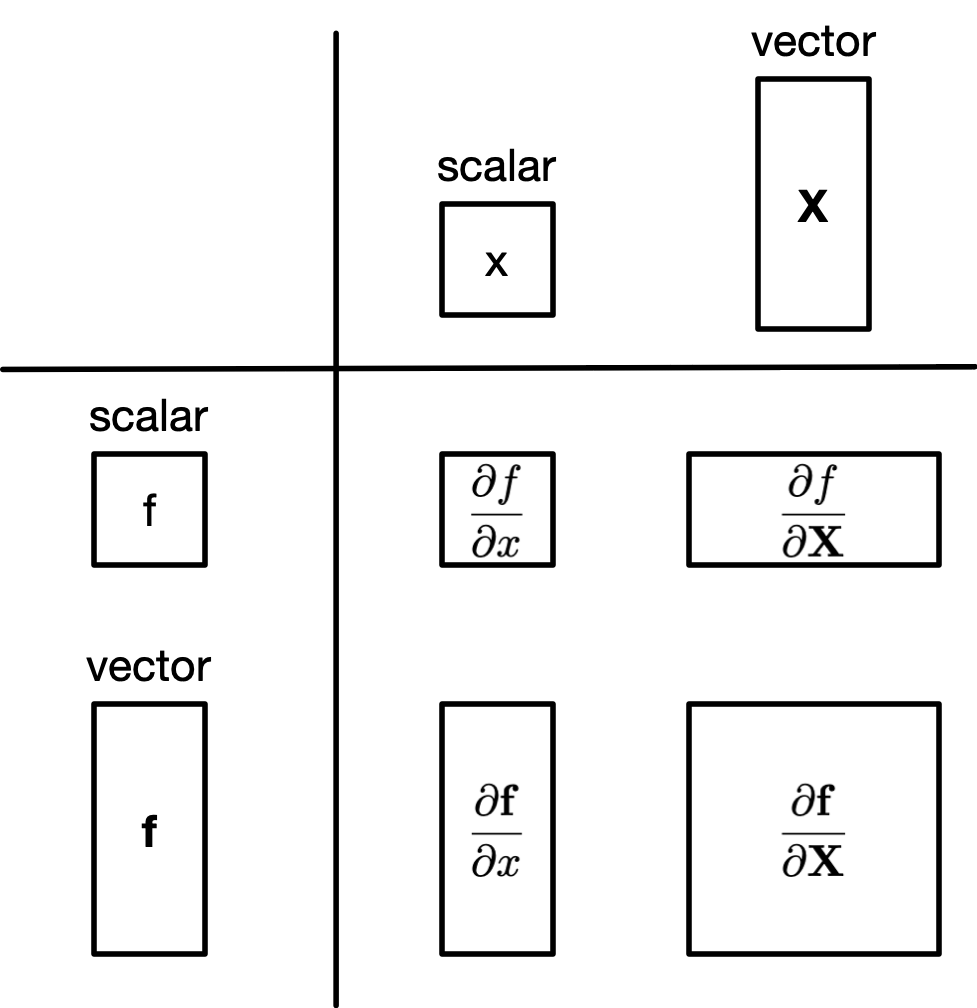
Q: Given a scalar $x$ and a vector of functions $f = \left[f_1, f_2, \ldots, f_n \right]$ what is $\frac{\partial f}{\partial x}$?
A: $\frac{\partial f}{\partial x} = \left[\frac{\partial f_1}{\partial x}, \frac{\partial f_2}{\partial x}, \ldots \frac{\partial f_n}{\partial x} \right]$
Q: Given a vector $X$ and a vector of functions $f = \left[f_1, f_2, \ldots, f_n \right]$ what is $\frac{\partial f}{\partial X}$?
A: $$ \frac{\partial f}{\partial X} = \begin{bmatrix} \nabla f_1(x) \ \nabla f_2(x) \ \vdots \ \nabla f_m(x)
= \begin{bmatrix} \frac{\partial}{\partial x_1} f_1(x) & \frac{\partial}{\partial x_2} f_1(x) & \dots & \frac{\partial}{\partial x_n} f_1(x) \\ \frac{\partial}{\partial x_1} f_2(x) & \frac{\partial}{\partial x_2} f_2(x) & \dots & \frac{\partial}{\partial x_n} f_2(x) \\ \vdots & \vdots & \ddots & \vdots \\ \frac{\partial}{\partial x_1} f_m(x) & \frac{\partial}{\partial x_2} f_m(x) & \dots & \frac{\partial}{\partial x_n} f_m(x) \end{bmatrix} $$
Q: Consider a matrix $A$ of size $m \times n$ and a vector $X$ of size $n \times 1$, what is $\frac{\partial AX}{\partial X}$?
Let's rewrite this a bit:
$$ AX = \begin{bmatrix} A_{11} x_1 + A_{12} x_2 + \dots + A_{1n} x_n\\ A_{21} x_1 + A_{22} x_2 + \dots + A_{2n} x_n\\ \vdots \\ A_{m1} x_1 + A_{m2} x_2 + \dots + A_{mn} x_n\\ \end{bmatrix} $$Another way to rewrite this:
$$ AX = \left[ \Sigma^n_{j=1} A_{1j} x_j, \Sigma^n_{j=1} A_{2j} x_j, \dots, \Sigma^n_{j=1} A_{mj} x_j \right] $$so
$$ (A X)_i = \sum_{j=1}^{n} A_{ij} x_j $$Now we can compute the derivative. Remember row is for each element of X and columns are for elements of $AX$:
$$ \frac{\partial}{\partial X} AX = \begin{bmatrix} \frac{\partial}{\partial x_1} \sum_{j=1}^{n} A_{1j} x_j & \frac{\partial}{\partial x_2} \sum_{j=1}^{n} A_{1j} x_j & \dots & \frac{\partial}{\partial x_n} \sum_{j=1}^{n} A_{1j} x_j \\ \frac{\partial}{\partial x_1} \sum_{j=1}^{n} A_{2j} x_j & \frac{\partial}{\partial x_2} \sum_{j=1}^{n} A_{2j} x_j & \dots & \frac{\partial}{\partial x_n} \sum_{j=1}^{n} A_{2j} x_j \\ \vdots & \vdots & \ddots & \vdots \\ \frac{\partial}{\partial x_1} \sum_{j=1}^{n} A_{mj} x_j & \frac{\partial}{\partial x_2} \sum_{j=1}^{n} A_{mj} x_j & \dots & \frac{\partial}{\partial x_n} \sum_{j=1}^{n} A_{mj} x_j \end{bmatrix} = \begin{bmatrix} A_{11} & A_{12} & \dots & A_{1n} \\ A_{21} & A_{22} & \dots & A_{2n} \\ \vdots & \vdots & \ddots & \vdots \\ A_{m1} & A_{m2} & \dots & A_{mn} \end{bmatrix} $$Q: What is the derivative of a vector with respect to itself ($f(x) = x$)
(and since $\frac{\partial}{\partial x_j} x_i = 0$ for $j \neq i$):
$$ = \begin{bmatrix} \frac{\partial}{\partial x_1} x_1 & 0 & \cdots & 0 \\ 0 & \frac{\partial}{\partial x_2} x_2 & \cdots & 0 \\ \vdots & \vdots & \ddots & \vdots \\ 0 & 0 & \cdots & \frac{\partial}{\partial x_n} x_n \end{bmatrix} = \begin{bmatrix} 1 & 0 & \cdots & 0 \\ 0 & 1 & \cdots & 0 \\ \vdots & \vdots & \ddots & \vdots \\ 0 & 0 & \cdots & 1 \end{bmatrix} = I \quad \text{(I is the identity matrix with ones down the diagonal)}. [2] $$The matrix calculations follow an intuitive pattern:
Alertness Check: Given two vectors $w$ and $x$ what is the hadamard product of the two vectors $\frac{\partial(w \otimes x)}{\partial x}$ with respect to x?
Some useful identities:
| Op | Partial with respect to $x$ | Partial with respect to $w$ |
|---|---|---|
| $$+$$ | $$\frac{\partial(w + x)}{\partial x} = I$$ | $$\frac{\partial(w + x)}{\partial w} = \text{diag}(1) = I$$ |
| $$-$$ | $$\frac{\partial(w - x)}{\partial x} = \text{diag}(-1) = -I$$ | $$\frac{\partial(w - x)}{\partial w} = \text{diag}(1) = I$$ |
| $$\otimes$$ | $$\frac{\partial(w \otimes x)}{\partial x} = \text{diag}(w)$$ | $$\frac{\partial(w \otimes x)}{\partial w} = \text{diag}(x)$$ |
| $$\oslash$$ | $$\frac{\partial(w / x)}{\partial x} = \text{diag}(-w / x^2)$$ | $$\frac{\partial(w / x)}{\partial w} = \text{diag}(1 / x)$$ |
Suppose we are summing two functions together $y=f(w) + g(x)$. $f$ and $g$ are both vectorized meaning $y$ looks like:
$$ \begin{bmatrix} y_1 \\ y_2 \\ \vdots \\ y_n \end{bmatrix} = \begin{bmatrix} f_1(\mathbf{w}) \circ g_1(\mathbf{x}) \\ f_2(\mathbf{w}) \circ g_2(\mathbf{x}) \\ \vdots \\ f_n(\mathbf{w}) \circ g_n(\mathbf{x}) \end{bmatrix} $$The Jacobian with respect to $w$ is:
$$ J_w = \frac{\partial y}{\partial w} = \begin{bmatrix} \frac{\partial}{\partial w_1} (f_1(w) \circ g_1(x)) & \frac{\partial}{\partial w_2} (f_1(w) \circ g_1(x)) & \cdots & \frac{\partial}{\partial w_n} (f_1(w) \circ g_1(x)) \\ \frac{\partial}{\partial w_1} (f_2(w) \circ g_2(x)) & \frac{\partial}{\partial w_2} (f_2(w) \circ g_2(x)) & \cdots & \frac{\partial}{\partial w_n} (f_2(w) \circ g_2(x)) \\ \vdots & \vdots & \ddots & \vdots \\ \frac{\partial}{\partial w_1} (f_n(w) \circ g_n(x)) & \frac{\partial}{\partial w_2} (f_n(w) \circ g_n(x)) & \cdots & \frac{\partial}{\partial w_n} (f_n(w) \circ g_n(x)) \end{bmatrix} $$and the Jacobian with respect to $x$ is:
$$ J_x = \frac{\partial y}{\partial x} = \begin{bmatrix} \frac{\partial}{\partial x_1} (f_1(w) \circ g_1(x)) & \frac{\partial}{\partial x_2} (f_1(w) \circ g_1(x)) & \cdots & \frac{\partial}{\partial x_n} (f_1(w) \circ g_1(x)) \\ \frac{\partial}{\partial x_1} (f_2(w) \circ g_2(x)) & \frac{\partial}{\partial x_2} (f_2(w) \circ g_2(x)) & \cdots & \frac{\partial}{\partial x_n} (f_2(w) \circ g_2(x)) \\ \vdots & \vdots & \ddots & \vdots \\ \frac{\partial}{\partial x_1} (f_n(w) \circ g_n(x)) & \frac{\partial}{\partial x_2} (f_n(w) \circ g_n(x)) & \cdots & \frac{\partial}{\partial x_n} (f_n(w) \circ g_n(x)) \end{bmatrix} $$Alertness Check: For what condition(s) and operation(s) are the off-diagonal components of $J_x = \frac{\partial f(x)}{\partial x} = 0$
$$ \frac{\partial y}{\partial x} = \begin{bmatrix} \frac{\partial}{\partial w_1} \left(f_1(w_1) \circ g_1(x_1)\right) & 0 & \cdots & 0 \\ 0 & \frac{\partial}{\partial w_2} \left(f_2(w_2) \circ g_2(x_2)\right) & \cdots & 0 \\ \vdots & \vdots & \ddots & \vdots \\ 0 & 0 & \cdots & \frac{\partial}{\partial w_n} \left(f_n(w_n) \circ g_n(x_n)\right) \end{bmatrix} $$When $f_i(w) = f_i(w_i)$, $g_i(x) = g_i(x_i)$, and $\circ$ is a element-wise operator.
Scalar expansion: $$\frac{\partial}{\partial x}fx = f $$
Vector sum reduction: $$ y = sum(X) $$
Let's reconsider the simple network we talked about in last lecture.
Remember we had a multi-function network:

Where the functions above are defined as follows:
$g(x) = x^2+1$, $h(g) = \log(g)$, $k(h) = \sin(h)$. Thus, $f(x) = k(h(g(x)))$
The resulting function is: $$f(x) = \sin(\log(((x)^2+1)))$$
One thing that bothers me about the previous flowchart is that $h$ and $k$ are single operators but $g$ is a complex function. As we know this isn't how PyTorch breaks down functions so let's fix this up quickly:
Where the functions above are defined as follows:
$e(x) = x^2$, $g(e) = e+1$, $h(g) = \log(g)$, $k(h) = \sin(h)$. Thus, $f(x) = k(h(g(x)))$
The resulting function is: $$f(x) = \sin(\log(((x)^2+1)))$$

At $x=1$, $\frac{\partial f}{\partial x} = \frac{2x\cos(\log(x^2+1))}{x^2+1} = .7692$ which we can verify with PyTorch:
import torch
import numpy

x = torch.Tensor([1])
x.requires_grad = True
e = x**2
g = e + 1
h = torch.log(g)
k = torch.sin(h)

# manual derivative (gradient)
with torch.no_grad():
    manual = 2*x*torch.cos(torch.log(x**2+1))/(x**2+1)

k.backward()
automatic = x.grad
print('Manually computed derivative from closed form: {}'.format(manual))
print('Letting PyTorch automatically find the derivative: {}'.format(automatic))
Manually computed derivative from closed form: tensor([0.7692])
Letting PyTorch automatically find the derivative: tensor([0.7692])
Pretty simple right? Ok let's change the above example a bit:
Where the functions above are defined as follows:
$e(x) = x^2$, $g(e,x) = e\mathbf{+x}$, $h(g) = \log(g)$, $k(h) = \sin(h)$. Thus, $f(x) = k(h(g(x)))$
The resulting function is: $$f(x) = \sin(\log(((x)^2+x)))$$
Since g is composed from two operations, let's take some partial derivatives:
$$ \begin{matrix} \frac{\partial}{\partial e}g(e,x) = 1 + 0 = 1 \frac{\partial}{\partial x}g(e,x) = 0 + 1 = 1 \end{matrix} $$So the question is what does \frac{df}{dx} look like:
Option 1: $$\frac{df}{dx} = \left.\frac{dk}{dh}\right|_{h(g)} \cdot \left.\frac{dh}{dg}\right|_{g(x)} \cdot \left.\frac{dg}{de}\right|_{e(x)} \cdot \left.\frac{de}{dx}\right|_x$$
$$\frac{df}{dx} = \cos(h(g)) \cdot \frac{1}{g(x)} \cdot 1 \cdot 2x = \cos(\log(x^2+1)) \cdot \frac{1}{x^2+1} \cdot 2x= \frac{2x\cos(\log(x^2+1))}{x^2+1}$$Option 2: $$\frac{df}{dx} = \left.\frac{dk}{dh}\right|_{h(g)} \cdot \left.\frac{dh}{dg}\right|_{g(x)} \cdot \left.\frac{dg}{dx}\right|_{x} $$
$$\frac{df}{dx} = \cos(h(g)) \cdot \frac{1}{g(x)} \cdot 1 \cdot 2x = \cos(\log(x^2+1)) \cdot \frac{1}{x^2+1} = \frac{\cos(\log(x^2+1))}{x^2+1}$$What's right? Well let's turn to PyTorch. At $x=1$ From the prior equations:
And PyTorch says:
import torch
import numpy

x = torch.Tensor([1])
x.requires_grad = True
e = x**2
g = e + x
h = torch.log(g)
k = torch.sin(h)

k.backward()
automatic = x.grad
print('Letting PyTorch automatically find the derivative: {}'.format(automatic))
Letting PyTorch automatically find the derivative: tensor([1.1539])
So neither option.... what's going on? Where's the error?
Since g is composed from two operations, let's take some partial derivatives:
$$ \begin{matrix} \frac{\partial}{\partial e}g(e,x) = 1 + 0 = 1 \mathbf{\frac{\partial}{\partial x}g(e,x) = 0 + 1 = 1} \end{matrix} $$The $\frac{\partial e}{\partial x} \neq 0$!

The law of total derivatives states that in ordercompute $\frac{\partial g(e,x)}{\partial x}$ we need to sum up all possibel contributions from $x$.
$$ \frac{d g(e,x)}{d x} = \frac{\partial g(e,x)}{\partial x} + \frac{\partial g(e,x)}{\partial e}\frac{\partial e(x)}{\partial x} $$Since g is composed from two operations, let's take some partial derivatives:
So the question is what does \frac{df}{dx} look like:
$$\frac{df}{dx} = \left.\frac{dk}{dh}\right|_{h(g)} \cdot \left.\frac{dh}{dg}\right|_{g(x)} \cdot \left(\left.\frac{dg}{de}\right|_{e(x)} \cdot \left.\frac{de}{dx}\right|_x + \left.\frac{dg}{dx}\right|_x \right)$$$$\frac{df}{dx} = \cos(h(g)) \cdot \frac{1}{g(x)} \cdot \left( 1 \cdot 2x + 1\right) = \cos(\log(x^2+1)) \cdot \frac{1}{x^2+1} \cdot \left( 2x + 1\right)= \frac{\left( 2x + 1\right)\cos(\log(x^2+1))}{x^2+1}$$At $x=1$, $\frac{df}{dx} = 1.1539$!
As we saw, calculuating the gradient relies on us knwoing exactly how inputs propogate through a computation. This is the exact reason for a computation graph.
New example:
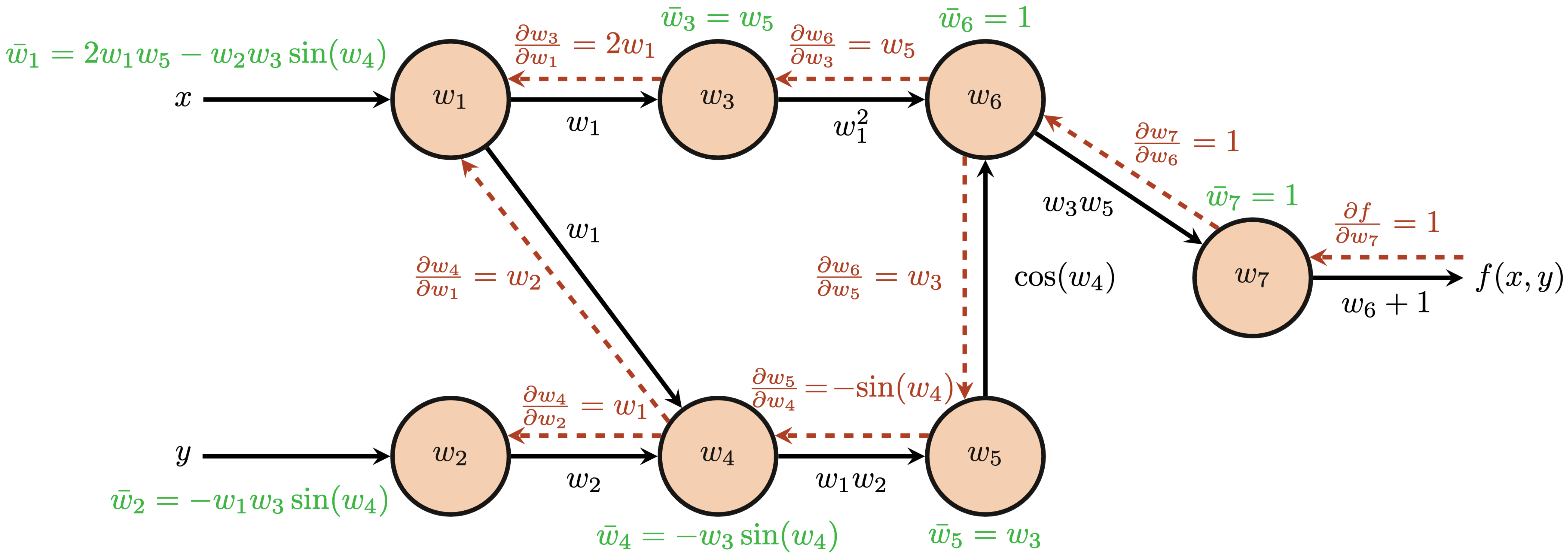
$$ \begin{align*} f(x, y) &= x^2\cos(xy)+1\\ f(x, y) &= f_1(f_2(f_3(x,y),f_4(f_5(x, y)))))\\ f_5(x, y) &= xy\\ f_4(f_5) &= \cos(f_5)\\ f_3(x, y) &= x^2\\ f_2(f_3, f_4) &= f_3f_4\\ f_1(f_2) &= f_2+1\\ f(x, y) &= f_1 \end{align*} $$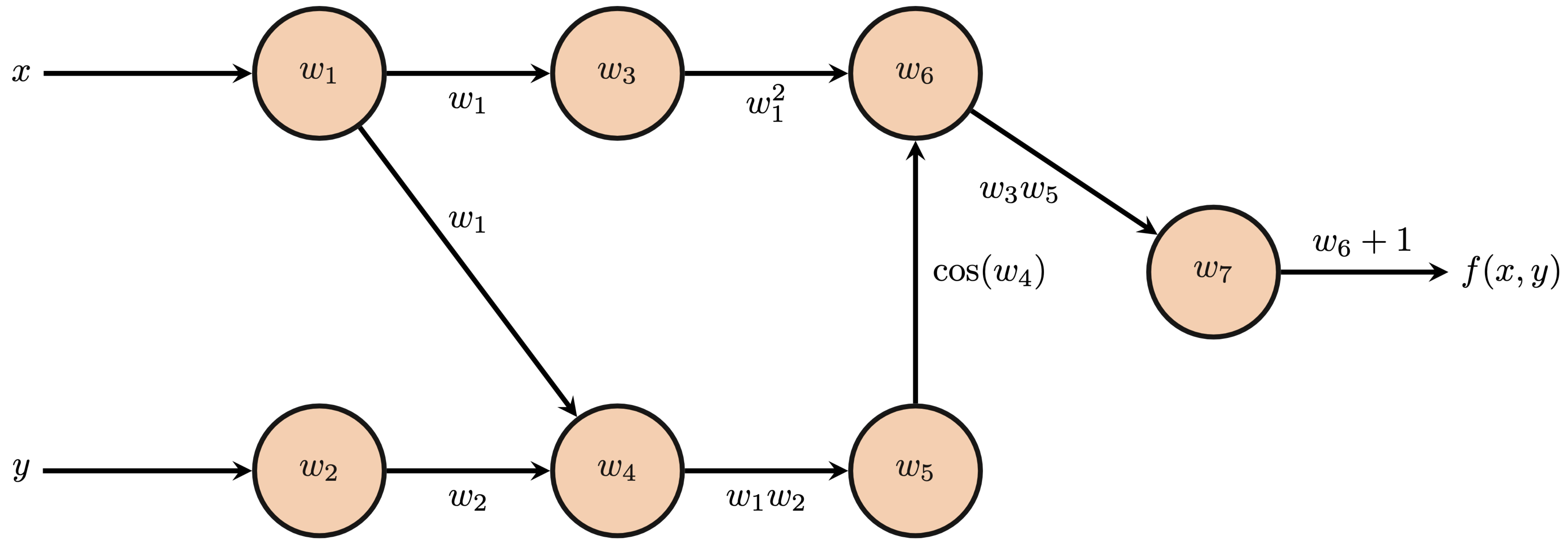
So the question, we want to make $f(x,y)$ to be 0. How should we change $x$/$y$ to minimize $f(x,y)$? What direction should we change each input?
Recall from prior lectures that knowing the gradient (derivative) can help us know which way to adjust the inputs. However, to callcuulate the gradient we need to know:
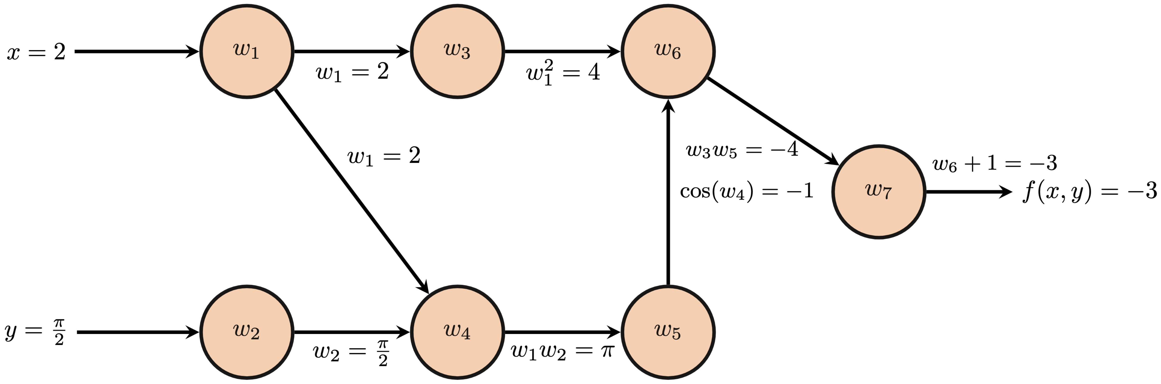
The forward pass through a computational graph is the direct calculation of applying the represented function to the provided inputs. Starting from every input node, $w_1$ and $w_2$ in our example, we follow each directed edge to the next node and perform the indicated operation to the available input(s) to generate the intermediate value at this next node. The next node then transmits this result to any of its successor nodes and so on until we reach any node(s) that have no successors. For the purposes of backpropagation, we refer to these end nodes with no successors as seed nodes. Below, we depict the forward pass through $f(x, y) = x^2\cos(xy)+1$ for $(x, y)=(2, \frac{\pi}{2})$.
After completing the forward pass, we now have exact values of the computation from each node. We also know the operation performed along each edge as each successor node may store the operation performed to obtain its result and the nodes for which it acts as the successor. For example, node $w_6$ performs the multiplication operation from nodes $w_3$ and $w_5$, i.e. $w_6=w_3w_5$. In summary, we have values at each node, operations at each node, and a directed acyclic graph structure which may be traversed backwards from each seed node.
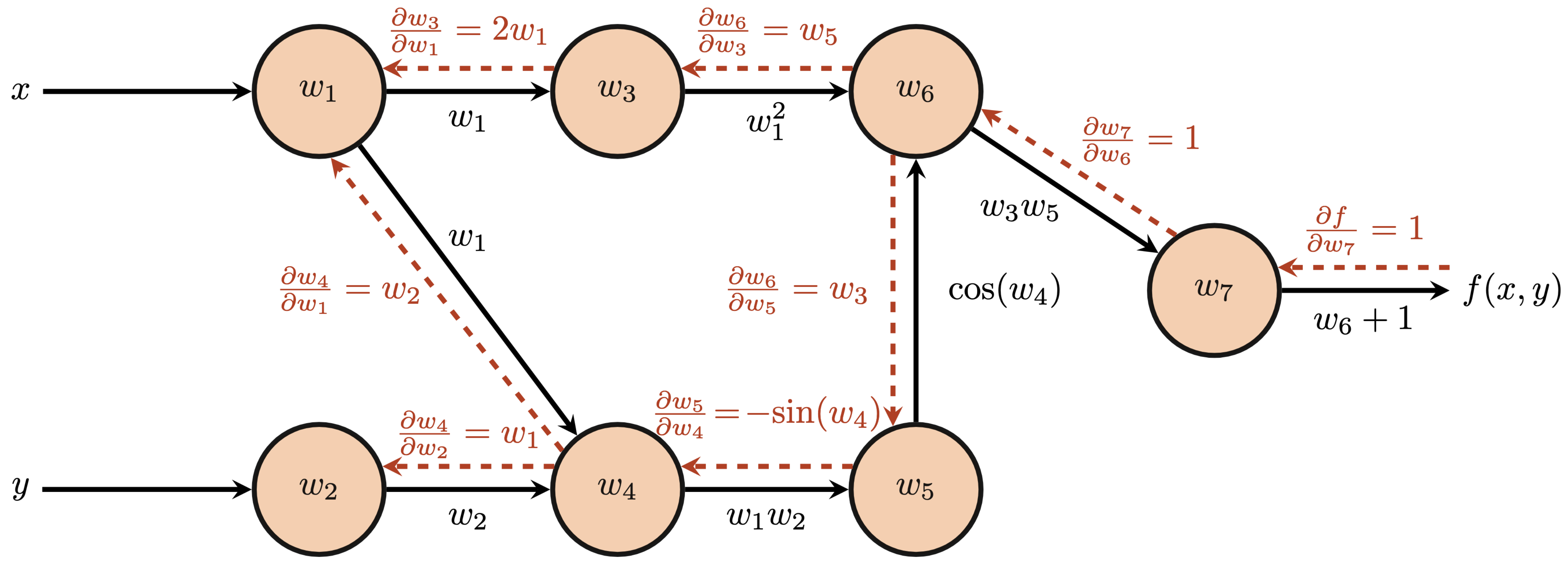
Propagating these partial derivatives and accumulating more complicated derivatives by chain rule at each node, however, still requires some coordination. We refer to these accumulated partial derivatives along the backward pass as the adjoint at each node and we denote the adjoint at node $i$ as $\bar{w}_i$. The adjoint at each node is calculated by
$$ \begin{align*} \bar{w}_i &= \frac{\partial f}{\partial w_i}\\ \bar{w}_i &= \sum_{j\in\textrm{successors}(w_i)}\bar{w}_j\frac{\partial w_j}{\partial w_i}. \end{align*} $$Let's compute the adjoint values for the above computational graph to gain some intuition for the above equations. We first have $\bar{w}_7$ as the "base case" since $f(x, y)=w_7$; thus, \begin{align*} \bar{w}_7 &= \frac{\partial f}{\partial w_7}\\ &=1. \end{align*}
Next, $w_7$ backpropagates to its predecessor $w_6$: \begin{align*} \bar{w}_6 &= \bar{w}_7\frac{\partial w_7}{\partial w_6}\\ &= \frac{\partial f}{\partial w_7}\frac{\partial w_7}{\partial w_6}\\ &= 1\\ \end{align*}
Altogether, we arrive at our final backpropagation results and final partial derivatives at the input nodes $\frac{\partial f}{\partial x}$ and $\frac{\partial f}{\partial y}$.
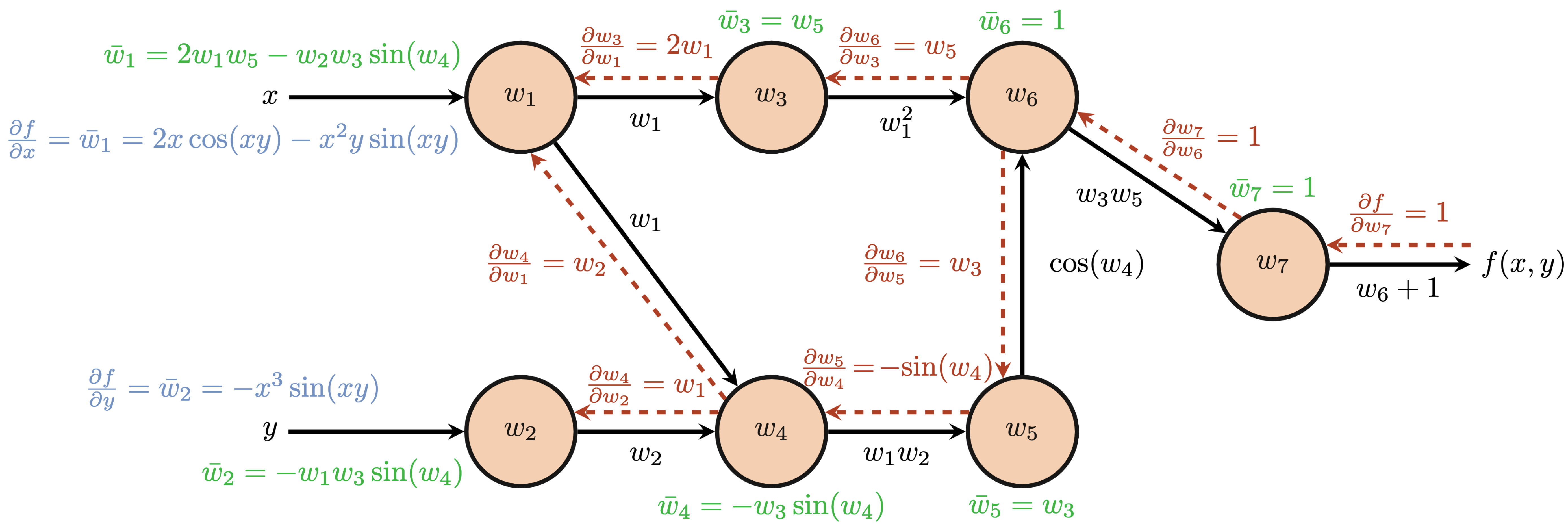
The entire procedure of backpropagation only requires one forward pass through the computational graph to establish the values at each node and one backward pass to accumulate gradients from seed nodes back through the entire graph. The backward pass is made significantly more efficient by the computed adjoint values that represent the accumulated gradients up to that node via chain rule. Each predecessor node re-uses the adjoint values of its successors and accumulates the partial derivatives of its successors with respect to itself. Thus, backpropagation may be seen as a form of dynamic programming as we recursively re-use previous computation for the next iteration or step of the algorithm.
import torch
import numpy as np

x = torch.tensor([float(-1)], requires_grad=True) # make sure gradients are computed when backpropagation is called
y = torch.tensor([np.pi/3], requires_grad=True)

w1 = x
w2 = y
w3 = w1**2
w4 = w1*w2
w5 = torch.cos(w4)
w6 = w3*w5
w7 = w6+1
f = w7

# manual gradients
with torch.no_grad():
    # adjoints
    w7bar = 1
    w6bar = 1
    w5bar = w3
    w4bar = -w3*torch.sin(w4)
    w3bar = w5
    w2bar = -w1*w3*torch.sin(w4)
    w1bar = 2*w1*w5 - w2*w3*torch.sin(w4)

# automatic gradients via backpropagation
w3.retain_grad(), w4.retain_grad(), w5.retain_grad(), w6.retain_grad(), w7.retain_grad() # making sure PyTorch populates all gradients
f.backward() # initiate backpropagation from f as the seed node

print('Comparing our calculations to PyTorch Autograd:')
print('w1: Manual = {}, PyTorch = {}'.format(w1bar, w1.grad))
print('w2: Manual = {}, PyTorch = {}'.format(w2bar, w2.grad))
print('w3: Manual = {}, PyTorch = {}'.format(w3bar, w3.grad))
print('w4: Manual = {}, PyTorch = {}'.format(w4bar, w4.grad))
print('w5: Manual = {}, PyTorch = {}'.format(w5bar, w5.grad))
print('w6: Manual = {}, PyTorch = {}'.format(w6bar, w6.grad))
print('w7: Manual = {}, PyTorch = {}'.format(w7bar, w7.grad))
Comparing our calculations to PyTorch Autograd:
w1: Manual = tensor([-0.0931]), PyTorch = tensor([-0.0931])
w2: Manual = tensor([-0.8660]), PyTorch = tensor([-0.8660])
w3: Manual = tensor([0.5000], grad_fn=<CosBackward0>), PyTorch = tensor([0.5000])
w4: Manual = tensor([0.8660]), PyTorch = tensor([0.8660])
w5: Manual = tensor([1.], grad_fn=<PowBackward0>), PyTorch = tensor([1.])
w6: Manual = 1, PyTorch = tensor([1.])
w7: Manual = 1, PyTorch = tensor([1.])
Next time we will be discussing gradient descent in great detail.
Suppose we have a function
$$ f(x) = \left[f_1(x), f_2(x)\right] $$
And a second 2-dimensional function: $$ g(y) = \left[g_1(y_1, y_2), g_2(y_1, y_2)\right] $$
Now let’s compose them to get:
$$ g(x) = [g_1(f_1(x), f_2(x)), g_2(f_1(x), f_2(x))] $$.
Using the regular chain rule, we can compute the derivative of $ g $ as the Jacobian
$$ \frac{\partial g}{\partial x} = \begin{bmatrix} \frac{\partial}{\partial x} g_1(f_1(x), f_2(x)) \\ \frac{\partial}{\partial x} g_2(f_1(x), f_2(x)) \end{bmatrix} = \begin{bmatrix} \frac{\partial g_1}{\partial y_1} \frac{\partial f_1}{\partial x} + \frac{\partial g_1}{\partial y_2} \frac{\partial f_2}{\partial x} \\ \frac{\partial g_2}{\partial y_1} \frac{\partial f_1}{\partial x} + \frac{\partial g_2}{\partial y_2} \frac{\partial f_2}{\partial x} \end{bmatrix} $$And we see this is the same as multiplying the two Jacobians: $$ \frac{\partial g}{\partial x} = \frac{\partial g}{\partial f} \frac{\partial f}{\partial x} = \begin{bmatrix} \frac{\partial g_1}{\partial f_1} & \frac{\partial g_1}{\partial f_2} \\ \frac{\partial g_2}{\partial f_1} & \frac{\partial g_2}{\partial f_2} \end{bmatrix} \begin{bmatrix} \frac{\partial f_1}{\partial x} \\ \frac{\partial f_2}{\partial x} \end{bmatrix} $$
[1]